Solving Systems of IVPs
Overview, Objectives, and Key Terms
The last lesson focused on one first-order initial-value problem at a time. Many useful models do not arrive that politely. A second-order spring equation, a set of coupled nuclide balances, and a spatial discretization of an ADR model all produce several unknowns that evolve together.
The move is simple: collect the unknowns into a state vector and solve one vector IVP.
By the end of this lesson, you should be able to
rewrite a higher-order ODE or coupled balance as a first-order system,
use forward and backward Euler on a linear system \(\mathbf{y}'=\mathbf{A}\mathbf{y}+\mathbf{s}\),
call
scipy.integrate.solve_ivpfor a system using the signaturef(t, y, ...), andcheck state ordering, output shapes, and active time scales.
Key terms: state vector, first-order system, forward Euler, backward Euler, stiffness, solve_ivp, t_eval.
[ ]:
import numpy as np
import matplotlib.pyplot as plt
from scipy.integrate import solve_ivp

PURPLE = "#512888"
ORANGE = "#D55E00"
BLUE = "#2563EB"
GREEN = "#059669"
RED = "#DC2626"
INK = "#1F2937"
MUTED = "#64748B"
GRID = "#E5E7EB"
PANEL = "#F5F6F8"

plt.rcParams.update({
    "figure.figsize": (7.2, 4.2),
    "axes.edgecolor": INK,
    "axes.labelcolor": INK,
    "xtick.color": INK,
    "ytick.color": INK,
    "grid.color": GRID,
})
A System Is One IVP With More Bookkeeping
A scalar IVP has the form
A system has the same structure, except the unknown is a vector:
This is exactly the same bookkeeping idea we used for finite-volume balances: decide what is being counted, put those quantities in a vector, and write a balance for each entry.
For a linear system, the right-hand side often looks like
where \(\mathbf{A}\) contains the coupling between unknowns and \(\mathbf{s}\) contains external sources.
From One Spring Equation to Two First-Order Equations
Consider a damped spring-mass system:
The model is second order because it contains \(x''\). To use Euler’s method or solve_ivp, we rewrite it as a first-order system. Define
Then
We will use the state ordering
which matches the worksheet. With that ordering,
[ ]:
# Input block: spring-mass parameters and state ordering.
k = 0.1   # spring constant
a = 0.2   # damping coefficient
m = 0.5   # mass
x0 = 0.0  # initial position
u0 = 1.0  # initial velocity

A = np.array([[0.0, 1.0],
              [-k/m, -a/m]])
y0 = np.array([x0, u0])

print("Input")
print(f"k={k:.3f}, a={a:.3f}, m={m:.3f}")
print(f"y0 = [x0, u0] = {y0}")
print("\nSystem matrix A:")
print(A)
Input
k=0.100, a=0.200, m=0.500
y0 = [x0, u0] = [0. 1.]

System matrix A:
[[ 0.   1. ]
 [-0.2 -0.4]]
The first row of \(\mathbf{A}\) says \(x'=u\). The second row says the velocity changes because the spring pulls back on the displacement and the damper pulls back on the velocity.
That row-level reading is worth keeping. A matrix row is not just algebra; it is a statement about how one state variable changes.
Euler Methods for a Linear System
For a scalar IVP, forward Euler uses the right-hand side at the old state. The vector version does the same thing:
For the linear homogeneous system \(\mathbf{y}'=\mathbf{A}\mathbf{y}\),
Backward Euler evaluates the right-hand side at the new state:
Move the unknown terms to the left:
That is the same lesson as our balance-law linear systems: reduce the step to algebra, then solve the algebra.
[ ]:
# One step of forward and backward Euler.
Delta = 0.5
I = np.eye(2)

y1_fe = (I + Delta*A) @ y0
y1_be = np.linalg.solve(I - Delta*A, y0)

print("Output")
print(f"forward Euler y1  = {y1_fe}")
print(f"backward Euler y1 = {y1_be}")
Output
forward Euler y1  = [0.5 0.8]
backward Euler y1 = [0.4 0.8]
Both methods are using the same model and the same time step. They differ in where they evaluate the slope. Forward Euler asks, “where would the old slope take me?” Backward Euler asks, “what new state is consistent with the new slope?”
[ ]:
def forward_euler_linear(A, y0, t):
    """Return states for y' = A y using forward Euler."""
    y = np.zeros((len(t), len(y0)))
    y[0] = y0
    for n in range(len(t) - 1):
        dt = t[n + 1] - t[n]
        y[n + 1] = (np.eye(len(y0)) + dt*A) @ y[n]
    return y


def backward_euler_linear(A, y0, t):
    """Return states for y' = A y using backward Euler."""
    y = np.zeros((len(t), len(y0)))
    y[0] = y0
    I = np.eye(len(y0))
    for n in range(len(t) - 1):
        dt = t[n + 1] - t[n]
        y[n + 1] = np.linalg.solve(I - dt*A, y[n])
    return y

# Time grid and numerical solutions.
t = np.linspace(0.0, 10.0, 21)
y_fe = forward_euler_linear(A, y0, t)
y_be = backward_euler_linear(A, y0, t)

print("Output")
print(f"y_fe shape: {y_fe.shape}")
print(f"y_be shape: {y_be.shape}")
print(f"last backward-Euler state [x, u]: {y_be[-1]}")
Output
y_fe shape: (21, 2)
y_be shape: (21, 2)
last backward-Euler state [x, u]: [-0.11808235 -0.07281104]
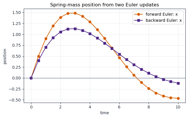
Our arrays are shaped (number of times, number of states). Column 0 is position \(x\) and column 1 is velocity \(u\). This is the shape many of our own loops naturally produce.
[ ]:
fig, ax = plt.subplots()
ax.plot(t, y_fe[:, 0], color=ORANGE, marker="o", label="forward Euler: x")
ax.plot(t, y_be[:, 0], color=PURPLE, marker="s", label="backward Euler: x")
ax.axhline(0.0, color=MUTED, lw=1)
ax.set_xlabel("time")
ax.set_ylabel("position")
ax.set_title("Spring-mass position from two Euler updates")
ax.grid(True, alpha=0.8)
ax.legend()
plt.show()
solve_ivp: The General-Purpose IVP Tool
For routine work, use scipy.integrate.solve_ivp. It expects the right-hand side in the order
def rhs(t, y, ...):
    return ...
This is an important detail. Older odeint examples often used f(y, t, ...); solve_ivp uses f(t, y, ...).
The core call is
sol = solve_ivp(rhs, t_span=(t0, tf), y0=y0, t_eval=t, args=(...))
where t_eval asks for output at the times we care about. Internally, the solver is free to take different steps.
[ ]:
def spring_rhs(t, y, k, a, m):
    """Right-hand side for y = [x, u]."""
    x, u = y
    return np.array([u, (-k*x - a*u)/m])

sol = solve_ivp(
    spring_rhs,
    t_span=(t[0], t[-1]),
    y0=y0,
    t_eval=t,
    args=(k, a, m),
    rtol=1e-9,
    atol=1e-11,
)

y_solve_ivp = sol.y.T
x_solve_ivp = y_solve_ivp[:, 0]
u_solve_ivp = y_solve_ivp[:, 1]

print("Output")
print(f"success: {sol.success}")
print(f"message: {sol.message}")
print(f"sol.y shape: {sol.y.shape}  (states, times)")
print(f"transposed shape: {y_solve_ivp.shape}  (times, states)")
print(f"last solve_ivp state [x, u]: {y_solve_ivp[-1]}")
Output
success: True
message: The solver successfully reached the end of the integration interval.
sol.y shape: (2, 21)  (states, times)
transposed shape: (21, 2)  (times, states)
last solve_ivp state [x, u]: [-0.2560552 -0.03725  ]
Notice the shape convention. solve_ivp returns sol.y with states along rows and times along columns. When we want the same shape as our Euler arrays, we use sol.y.T.
[ ]:
fig, ax = plt.subplots()
ax.plot(t, y_be[:, 0], color=PURPLE, marker="s", label="backward Euler: x")
ax.plot(t, x_solve_ivp, color=INK, lw=2.2, label="solve_ivp: x")
ax.plot(t, y_be[:, 1], color=ORANGE, marker="o", label="backward Euler: u")
ax.plot(t, u_solve_ivp, color=BLUE, lw=2.2, label="solve_ivp: u")
ax.axhline(0.0, color=MUTED, lw=1)
ax.set_xlabel("time")
ax.set_ylabel("state value")
ax.set_title("Backward Euler and solve_ivp solve the same system")
ax.grid(True, alpha=0.8)
ax.legend(ncol=2)
plt.show()
[ ]:
# Output/check block: compare backward Euler to solve_ivp on the same output grid.
error = y_be - y_solve_ivp
max_position_error = np.max(np.abs(error[:, 0]))
max_velocity_error = np.max(np.abs(error[:, 1]))

print("Output/check")
print(f"max |x_BE - x_solve_ivp| = {max_position_error:.4e}")
print(f"max |u_BE - u_solve_ivp| = {max_velocity_error:.4e}")
print(f"first requested time: {sol.t[0]:.1f}, last requested time: {sol.t[-1]:.1f}")
Output/check
max |x_BE - x_solve_ivp| = 1.5559e-01
max |u_BE - u_solve_ivp| = 8.9837e-02
first requested time: 0.0, last requested time: 10.0
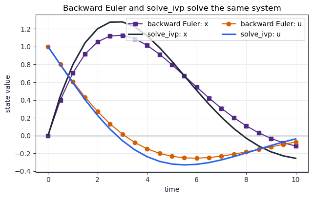
The backward-Euler result is a valid numerical solution, but it uses a deliberately coarse time step. solve_ivp adjusts internal steps to meet error tolerances, then reports the solution at the requested t_eval times.
That distinction is central: t_eval controls output times, not necessarily every internal step the solver takes.
A Fast/Slow Balance System
Systems become more interesting when different state variables evolve on different time scales. A simple linear production-decay chain is
Here \(n_1\) is produced directly, \(n_1\) feeds \(n_2\), and \(n_2\) decays slowly. If \(\lambda_1\) is much larger than \(\lambda_2\), then the first component moves quickly while the second component drifts slowly.
[ ]:
# Input block: a fast/slow linear balance system.
lambda1 = 10.0
lambda2 = 0.01
q = 1.0
z0 = np.array([0.0, 0.0])
A_chain = np.array([[-lambda1, 0.0],
                    [ lambda1, -lambda2]])
s_chain = np.array([q, 0.0])
t_chain = np.linspace(0.0, 500.0, 400)

print("Input")
print(f"lambda1={lambda1:g}, lambda2={lambda2:g}, q={q:g}")
print("A_chain =")
print(A_chain)
print(f"source = {s_chain}")
Input
lambda1=10, lambda2=0.01, q=1
A_chain =
[[-10.     0.  ]
 [ 10.    -0.01]]
source = [1. 0.]
[ ]:
def chain_rhs(t, z, lambda1, lambda2, q):
    n1, n2 = z
    return np.array([q - lambda1*n1, lambda1*n1 - lambda2*n2])

sol_rk = solve_ivp(
    chain_rhs,
    (t_chain[0], t_chain[-1]),
    z0,
    t_eval=t_chain,
    args=(lambda1, lambda2, q),
    rtol=1e-7,
    atol=1e-10,
    method="RK45",
)

sol_bdf = solve_ivp(
    chain_rhs,
    (t_chain[0], t_chain[-1]),
    z0,
    t_eval=t_chain,
    args=(lambda1, lambda2, q),
    rtol=1e-7,
    atol=1e-10,
    method="BDF",
)

print("Output")
print(f"RK45 success={sol_rk.success}, function calls={sol_rk.nfev}")
print(f"BDF  success={sol_bdf.success}, function calls={sol_bdf.nfev}")
print(f"final BDF state [n1, n2] = {sol_bdf.y[:, -1]}")
Output
RK45 success=True, function calls=10778
BDF  success=True, function calls=478
final BDF state [n1, n2] = [ 0.1       99.3255131]
[ ]:
fig, (ax0, ax1) = plt.subplots(1, 2, figsize=(10.2, 3.9), constrained_layout=True)

ax0.plot(sol_bdf.t, sol_bdf.y[0], color=PURPLE, label="$n_1$ fast")
ax0.plot(sol_bdf.t, sol_bdf.y[1], color=ORANGE, label="$n_2$ slow")
ax0.set_xlabel("time")
ax0.set_ylabel("inventory")
ax0.set_title("Both states")
ax0.grid(True, alpha=0.8)
ax0.legend()

ax1.plot(sol_bdf.t, sol_bdf.y[0], color=PURPLE, label="$n_1$")
ax1.set_xlim(0, 2.0)
ax1.set_xlabel("time")
ax1.set_ylabel("inventory")
ax1.set_title("Fast transient detail")
ax1.grid(True, alpha=0.8)
ax1.legend()

plt.show()
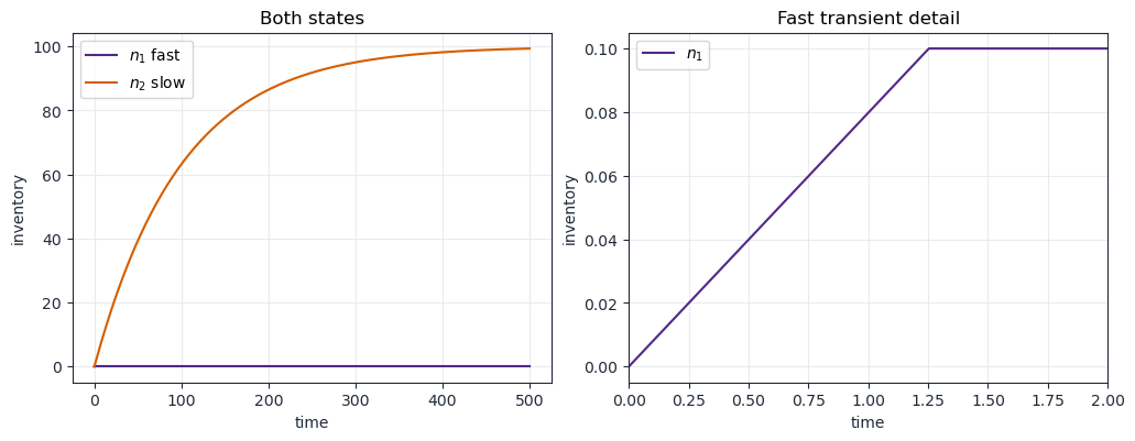
The first inventory reaches its near-steady value quickly. The second inventory changes on a much longer time scale. That spread in time scales is the practical warning sign for stiffness.
solve_ivp lets us choose methods explicitly. RK45 is a good default for many non-stiff problems. BDF is built for stiff systems. The point here is not to memorize method internals; it is to recognize when a model contains fast and slow balances in the same state vector.
What To Check Every Time
After solving a system IVP, check the bookkeeping before trusting the curve.
State order: Is the vector really
[x, u],[n1, n2], or whatever the model statement says?Right-hand-side signature: For
solve_ivp, did you writef(t, y, ...)?Array shape:
sol.yis(number of states, number of output times). Transpose it when you want rows to correspond to times.Solver status: Is
sol.successtrue, and does the message make sense?Time scales and units: Does the result move on the expected time scale, and do the signs match the balance?
The computational pattern is short:
def rhs(t, y, ...):
    ...
    return dydt

sol = solve_ivp(rhs, (t0, tf), y0, t_eval=t, args=(...))
y_by_time = sol.y.T
The engineering work is deciding what belongs in the state vector and what each row of the derivative means.
Further Reading
SciPy documentation for
`solve_ivp<https://docs.scipy.org/doc/scipy/reference/generated/scipy.integrate.solve_ivp.html>`__SciPy user guide section on integrating ordinary differential equations
Previous lessons: finite-volume bookkeeping in L10, ADR balances in L26, symbolic IVP scaffolds in L27, and scalar Euler methods in L28.