Lesson 13 - Symbolic Computation with SymPy

Learning goals. By the end of this lecture, students will be able to:

• define symbolic variables, expressions, equations, vectors, and matrices in SymPy,

• solve small linear systems symbolically and interpret the resulting formulas,

• use SymPy notebooks to carry multi-step symbolic analysis,

• turn symbolic expressions into LaTeX strings, numerical functions, and plots,

• compare symbolic and numerical workflows,

• verify small-system algebra before applying the same model idea at larger scale.

Key terms. symbolic variable, symbolic expression, SymPy, simplification, symbolic solve, lambdify.

Why symbolic computation belongs here

In the last several chapters, the work has mostly been numerical: assemble \(\mathbf{A}\), solve \(\mathbf{A}\mathbf{x}=\mathbf{b}\), and check the residual. That is still the right workflow for realistic models. But there is one piece of work that often happens before the numbers arrive: the formula deserves a look before it turns into code.

This is where SymPy earns its place. It lets a notebook carry the algebra that would otherwise sprawl across a page of scratch work. The point is not to make the computer think for us. The point is to ask better questions while the symbols are still visible: What assumptions are hidden in this formula? How does the response depend on a parameter? What expression belongs in documentation, plots, or numerical evaluation?

Symbolic computation is useful when the task is to:

• carry out algebraic analysis without pages of handwritten manipulation,

• derive a model coefficient from parameters,

• simplify a small system before coding a larger one,

• check algebra that would otherwise be done by hand,

• understand how a solution depends on a parameter,

• generate a LaTeX expression for documentation,

• generate an expression that can later be plotted or evaluated numerically.

So the default split is simple: use SymPy when the small model or derivation is trying to tell you something, then turn the result back into numerical code when the problem gets large. Symbolic work gives us a better view of the assumptions; numerical work remains the way we solve realistic engineering systems.

Example.

A symbolic :math:`2times 2` solve shows what the matrix entries are doing. Before we attach a matrix to a physical model, it is useful to see the plain algebra. Let

\[\begin{split}\mathbf{A}= \begin{bmatrix} a_{11} & a_{12}\\ a_{21} & a_{22} \end{bmatrix}, \qquad \mathbf{b}= \begin{bmatrix} b_1\\ b_2 \end{bmatrix}.\end{split}\]

Solving \(\mathbf{A}\mathbf{x}=\mathbf{b}\) symbolically gives

\[x_1=\frac{a_{22}b_1-a_{12}b_2}{a_{11}a_{22}-a_{12}a_{21}}, \qquad x_2=\frac{-a_{21}b_1+a_{11}b_2}{a_{11}a_{22}-a_{12}a_{21}}.\]

The denominator is the determinant. When the matrix entries change, the solution changes through both the numerator and this shared denominator.

Listing. Solving a general symbolic 2-by-2 system.

import sympy as sp

a11, a12, a21, a22, b1, b2 = sp.symbols("a11 a12 a21 a22 b1 b2")
A = sp.Matrix([[a11, a12],
               [a21, a22]])
b = sp.Matrix([b1, b2])
x = sp.simplify(A.LUsolve(b))
detA = sp.factor(A.det())

print(detA)
print(x)

case_uncoupled = x.subs({a11: 2, a12: 0,  a21: 0,  a22: 3, b1: 1, b2: 1})
case_coupled   = x.subs({a11: 2, a12: -1, a21: -1, a22: 3, b1: 1, b2: 1})
case_weak_diag = x.subs({a11: 2, a12: -1, a21: -1, a22: sp.Rational(6, 5),
                         b1: 1, b2: 1})

a11*a22 - a12*a21
Matrix([[(-a12*b2 + a22*b1)/(a11*a22 - a12*a21)], [(a11*b2 - a21*b1)/(a11*a22 - a12*a21)]])

For these three substitutions, the same symbolic formula gives

\[\begin{split}\begin{array}{c|c} \text{matrix choice} & \mathbf{x}\\ \hline \begin{bmatrix}2&0\\0&3\end{bmatrix} & \begin{bmatrix}1/2\\1/3\end{bmatrix}\\[0.8em] \begin{bmatrix}2&-1\\-1&3\end{bmatrix} & \begin{bmatrix}4/5\\3/5\end{bmatrix}\\[0.8em] \begin{bmatrix}2&-1\\-1&6/5\end{bmatrix} & \begin{bmatrix}11/7\\15/7\end{bmatrix} \end{array}\end{split}\]

The right-hand side is the same in all three cases. The solution changes because the operator changed: coupling terms move response between unknowns, and a smaller determinant amplifies the result. This is exactly the kind of behavior we want to see before hiding the formula inside a numerical solve.

Symbols and expressions

In NumPy, a variable usually stores a value. In SymPy, a variable can store a mathematical symbol.

Listing. Defining symbols and expressions in SymPy.

import sympy as sp
sp.init_printing()

c, s1, s2 = sp.symbols('c s1 s2')
expr = s1 + c*s2/2
print(expr)

c*s2/2 + s1

The object expr is not yet a floating-point number. It is the symbolic expression

\[s_1+\frac{c s_2}{2}.\]

We can substitute values later:

expr_num = expr.subs({c: 0.8, s1: 1.0, s2: 0.0})
print(expr_num)
print(expr_num.evalf())

1.00000000000000
1.00000000000000

Equations are not assignments

This is the small trap worth fixing early. In Python, the statement E = m*c**2 assigns an expression to a name. It does not create a mathematical equation to be solved. In SymPy, equations are created with Eq.

Listing. Creating and solving a symbolic equation.

m, speed, E = sp.symbols('m speed E')
eq = sp.Eq(E, m*speed**2)
sol_m = sp.solve(eq, m)
print(sol_m)

[E/speed**2]

This solves

\[E=m\,\text{speed}^2\]

for \(m\), giving

\[m=\frac{E}{\text{speed}^2}.\]

A good habit is to tell solve exactly which symbol or symbols are the unknowns. This avoids ambiguity in systems with many parameters.

A two-cell symbolic balance model

Consider a two-cell version of the fixed-step walk from Lesson 10. Let \(x_1\) and \(x_2\) be the steady populations, let \(s_1\) and \(s_2\) be external sources, and let \(c\) be the survival-and-scattering fraction. The balances are

\[x_1 = s_1 + \frac{c}{2}x_2,\]

\[x_2 = s_2 + \frac{c}{2}x_1.\]

Move unknowns to the left:

\[\begin{split}\begin{bmatrix} 1 & -c/2\\ -c/2 & 1 \end{bmatrix} \begin{bmatrix}x_1\\x_2\end{bmatrix} = \begin{bmatrix}s_1\\s_2\end{bmatrix}.\end{split}\]

This system is small enough to solve symbolically, which means we can ask what the parameters are doing before we commit to one numerical case.

Listing. Solving a symbolic two-cell balance model.

c, s1, s2 = sp.symbols('c s1 s2')
x1, x2 = sp.symbols('x1 x2')

A = sp.Matrix([[1, -c/2],
               [-c/2, 1]])
x = sp.Matrix([x1, x2])
b = sp.Matrix([s1, s2])

sol = sp.solve(sp.Eq(A*x, b), (x1, x2), dict=True)[0]
print(sp.simplify(sol[x1]))
print(sp.simplify(sol[x2]))

2*(-c*s2 - 2*s1)/(c**2 - 4)
2*(-c*s1 - 2*s2)/(c**2 - 4)

The solution is

\[x_1 = \frac{s_1+\frac{c}{2}s_2}{1-\frac{c^2}{4}},\]

\[x_2 = \frac{\frac{c}{2}s_1+s_2}{1-\frac{c^2}{4}}.\]

Now the formula is doing more than returning two answers. It shows parameter dependence that a single numerical solve would hide. The denominator \(1-c^2/4\) says that the two-cell response becomes more amplified as \(c\) increases. In the physical interpretation here, \(c\) is a survival-and-scattering fraction, so the usual sweep is \(0 \leq c \leq 1\). Algebraically, the same denominator also warns that \(c=\pm 2\) would make the formula break down. Those values are not plausible survival fractions in this model; they are the symbolic restriction the algebra exposed for us.

Example.

Reading a formula as an engineering warning. Set \(s_1=1\) and \(s_2=0\). The symbolic result gives

\[x_1(c)=\frac{1}{1-c^2/4}, \qquad x_2(c)=\frac{c/2}{1-c^2/4}.\]

When \(c=0\), no population scatters from cell to cell, so \(x_1=1\) and \(x_2=0\). When \(c=0.8\), the response becomes

\[x_1=\frac{25}{21}\approx 1.19, \qquad x_2=\frac{10}{21}\approx 0.476.\]

The symbolic expression explains the numerical trend: increasing \(c\) shrinks the denominator and amplifies the response, while also moving some of the source response into the neighboring cell. This is the kind of information a single numerical solve does not automatically reveal.

Matrix methods in SymPy

SymPy matrices also provide methods that look like linear algebra. That is useful because the symbolic workflow can mirror the numerical workflow from Lesson 12: build \(\mathbf{A}\), build \(\mathbf{b}\), solve \(\mathbf{A}\mathbf{x}=\mathbf{b}\), and then inspect the result. The difference is that the result is a formula, so inspection matters more, not less.

Listing. Using SymPy matrix solve routines.

x_symbolic = A.LUsolve(b)
print(sp.simplify(x_symbolic[0]))
print(sp.simplify(x_symbolic[1]))

2*(-c*s2 - 2*s1)/(c**2 - 4)
2*(-c*s1 - 2*s2)/(c**2 - 4)

The method name LUsolve is a useful reminder that solving a linear system is often organized through a factorization. For symbolic matrices, the output is a formula. For numerical matrices, the output is a numerical vector.

Because this system is only \(2\times 2\), it is also useful to inspect the inverse symbolically:

Listing. Inspecting the inverse of the two-cell matrix.

A_inv = sp.simplify(A.inv())
print(A_inv)
print(sp.simplify(A_inv*b))

Matrix([[-4/(c**2 - 4), -2*c/(c**2 - 4)], [-2*c/(c**2 - 4), -4/(c**2 - 4)]])
Matrix([[2*(-c*s2 - 2*s1)/(c**2 - 4)], [2*(-c*s1 - 2*s2)/(c**2 - 4)]])

SymPy gives

\[\begin{split}\mathbf{A}^{-1} = \frac{1}{1-c^2/4} \begin{bmatrix} 1 & c/2\\ c/2 & 1 \end{bmatrix}.\end{split}\]

Multiplying this inverse by \(\mathbf{b}=[s_1,s_2]^\mathsf{T}\) produces the same formulas for \(x_1\) and \(x_2\). The inverse is not a recommendation for large numerical work. Here it is a small symbolic object that shows exactly where the shared denominator enters the response.

Substitution and numerical evaluation

Once a symbolic formula is derived, we can evaluate it for specific parameter values. If \(s_1=1\), \(s_2=0\), and \(c=0.8\), the two-cell solution becomes

Listing. Substituting numbers into a symbolic solution.

values = {s1: 1.0, s2: 0.0, c: 0.8}
x1_num = sol[x1].subs(values).evalf()
x2_num = sol[x2].subs(values).evalf()
print(x1_num, x2_num)

1.19047619047619 0.476190476190476

The exact symbolic expressions are useful for derivation. The evaluated numbers are useful for computation and interpretation.

Example.

Checking a symbolic formula against a numerical residual. After substituting numerical values, check the equation \(\mathbf{A}\mathbf{x}=\mathbf{b}\). For \(s_1=1\), \(s_2=0\), and \(c=0.8\),

\[\begin{split}\mathbf{A}= \begin{bmatrix} 1 & -0.4\\ -0.4 & 1 \end{bmatrix}, \qquad \mathbf{x}= \begin{bmatrix} 25/21\\ 10/21 \end{bmatrix}.\end{split}\]

Then

\[\mathbf{b}-\mathbf{A}\mathbf{x}=\mathbf{0}.\]

This check matters because symbolic work can produce a formula that is algebraically correct but still used with the wrong substitution, wrong variable order, or wrong sign convention. The residual test catches those implementation mistakes.

Simplify, expand, factor, and collect

Symbolic expressions can often be written in several equivalent forms. SymPy provides tools for moving among those forms.

Listing. Equivalent forms of symbolic expressions.

z, alpha = sp.symbols('z alpha')

den = 1 - z**2/4
print(sp.factor(den))
print(sp.expand((1 - z/2)*(1 + z/2)))

messy = (z**2 - 4)/(z - 2)
print(sp.simplify(messy))

poly = sp.expand((1 + alpha*z)*(1 + z + z**2))
print(sp.collect(poly, z))

-(z - 2)*(z + 2)/4
1 - z**2/4
z + 2
alpha*z**3 + z**2*(alpha + 1) + z*(alpha + 1) + 1

Common operations include:

• simplify: attempt to find a simpler equivalent expression,

• expand: multiply out products,

• factor: factor polynomials when possible,

• collect: group terms by powers of a chosen symbol.

These tools are helpful, but they are not magic. Factored form can expose parameter values that require caution. Expanded form can show individual powers. Collected form can group terms by the symbol we want to study. A simplified form may be shorter, but shorter is not always clearer; for example, simplifying \((z^2-4)/(z-2)\) hides the fact that the original expression had a denominator. The working habit is to inspect symbolic output rather than accepting it uncritically.

Turning symbolic expressions into numerical functions

A symbolic expression can be converted into a numerical Python function using lambdify. This is useful for plotting or for evaluating a derived coefficient many times.

Listing. Converting a symbolic expression to a numerical function.

x1_expr = sp.simplify(sol[x1].subs({s1: 1, s2: 0}))
print(sp.latex(x1_expr))

x1_fun = sp.lambdify(c, x1_expr, 'numpy')
print(x1_fun(0.8))

- \frac{4}{c^{2} - 4}
1.1904761904761905

The latex output can be used in notes, reports, or figure labels. Passing 'numpy' to lambdify makes array evaluation explicit, which is what we usually want for parameter sweeps and plots.

Example.

A symbolic-to-numeric parameter sweep. The lambdified function can be evaluated on a grid of \(c\) values. A few values already give useful intuition:

import numpy as np
import matplotlib.pyplot as plt

c_values = np.linspace(0.0, 0.99, 100)
x1_values = x1_fun(c_values)

fig, ax = plt.subplots()
ax.plot(c_values, x1_values)
ax.set_xlabel('coupling c')
ax.set_ylabel('x1(c)')
ax.grid(True)

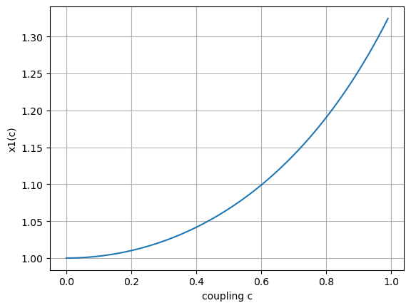
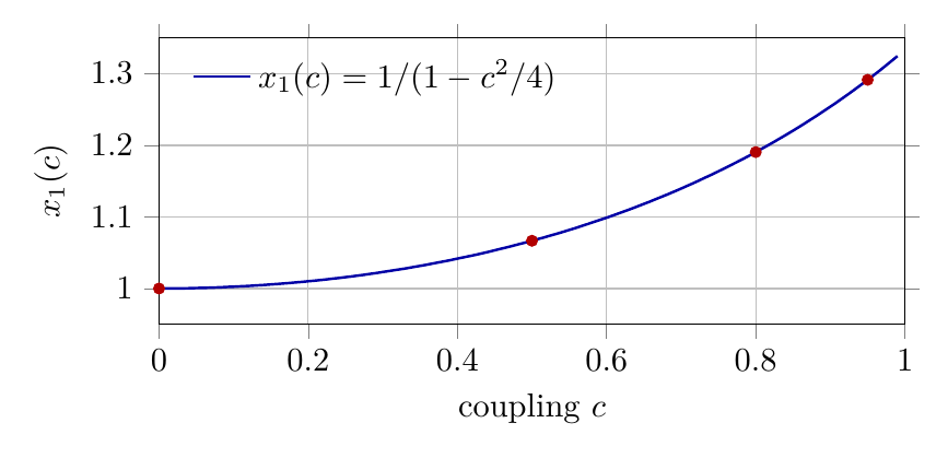
Figure. The lambdified symbolic expression \(x_1(c)=1/(1-c^2/4)\) evaluated over a coupling sweep.

\[\begin{split}\begin{aligned} x_1(0.0) &= 1.000,\\ x_1(0.5) &\approx 1.067,\\ x_1(0.8) &\approx 1.190,\\ x_1(0.95) &\approx 1.291. \end{aligned}\end{split}\]

The point of the table or plot is not the arithmetic; it is the workflow. SymPy derives the expression once, and NumPy evaluates the expression many times. That same pattern is useful when a coefficient, response factor, or limiting expression must be derived before being used in a numerical model.

Symbolic versus numerical workflows

Symbolic and numerical workflows answer different questions.

A symbolic workflow asks:

• Can I use the notebook to carry the algebra instead of spreading it across pages?

• Can I derive a formula?

• How does the answer depend on parameters?

• Can I simplify, document, plot, or evaluate the result before implementing it numerically?

A numerical workflow asks:

• What is the answer for this specific case?

• How do I solve a large system efficiently?

• How small is the residual?

For small systems, symbolic computation can reveal structure. It can also reveal assumptions: denominators that must not vanish, parameter ranges where a formula changes behavior, and limiting cases where the model stops making physical sense. For large systems, symbolic formulas become too large to be useful, and numerical methods are preferred.

Verifying algebra before scaling up. The two-cell model is not the final engineering model. It is a small test case. If the symbolic two-cell derivation matches the row-by-row balance logic, then the same pattern can be extended to many cells with more confidence.

This is a common strategy:

1. derive a small symbolic version,

2. check the formula against physical intuition,

3. substitute numerical values and compare with a numerical solve,

4. scale the same assembly pattern to a larger numerical matrix.

Exercises

1. In SymPy, define symbols \(a\), \(b\), and \(x\). Write the symbolic expression \(a x+b\), then substitute \(a=2\), \(b=-1\), and \(x=3\). What symbolic expression and value do you get?

2. Solve the symbolic equation \(p y+q=0\) for \(y\). What assumption about \(p\) is implicit in the formula?

3. For the two-cell balance model with \(s_1=1\), \(s_2=0\), and symbolic coupling \(c\), use the formula from the chapter to write \(x_1(c)\). Evaluate it at \(c=0\) and \(c=0.8\).

4. Explain why a symbolic two-cell derivation is useful even when the final engineering model will be solved numerically with many cells.

5. Factor the denominator \(1-c^2/4\). What parameter values does this form flag?

6. What are two practical uses for sp.latex and sp.lambdify after deriving \(x_1(c)\)?

Answers.

1. The symbolic expression is \(a x+b\). After substitution, it becomes \(2(3)-1=5\).

2. The solution is \(y=-q/p\). This assumes \(p\neq 0\).

3. The first-cell response is

   \[x_1(c)=\frac{1}{1-c^2/4}.\]

Thus \(x_1(0)=1\), and

\[x_1(0.8)=\frac{1}{1-0.16}=\frac{25}{21}\approx 1.1905.\]

1. The small symbolic model checks the algebra, exposes parameter dependence, and confirms the row pattern before the same assembly idea is scaled to a larger numerical matrix.

2. The denominator factors as \((1-c/2)(1+c/2)\), or equivalently \(-\frac{1}{4}(c-2)(c+2)\). It flags \(c=2\) and \(c=-2\).

3. sp.latex turns the expression into documentation-ready math, and sp.lambdify turns it into a numerical function for repeated evaluation or plotting.

End-of-lecture summary

Takeaway.

• SymPy carries notebook algebra; NumPy handles large numerical cases.

• Eq states an equation; assignment names an object.

• Small symbolic systems reveal parameter dependence and hidden assumptions.

• latex and lambdify turn one formula into documentation, plots, and checks.

• Lesson 14 returns to large systems: residuals, sparsity, and iteration.