Numerical Differentiation
Overview, Objectives, and Key Terms
From Lecture 1 through the first half of the course, we used Python to assemble models, solve linear systems, check residuals, and interpret response quantities. We now shift toward numerical calculus: computing derivatives from formulas, black-box functions, or sampled data.
In this lesson, we use Taylor series to derive finite-difference approximations for derivatives, then compare three practical derivative estimates: forward/backward differences, central differences, and the complex-step method. We finish by moving from a one-dimensional derivative to the gradient of a scalar field, which is the derivative object we need for many balance-law and transport applications.
We will use the symbol \(\Delta\) in formulas and Delta in code for the finite-difference step.
Objectives
By the end of this lesson, you should be able to
Derive first- and second-derivative finite-difference approximations using Taylor series.
Explain the difference between truncation error and floating-point roundoff error.
Compare forward, backward, central, and complex-step derivative estimates for a callable function.
Estimate a gradient from sampled two-dimensional data using
np.gradient.Use plots as evidence for accuracy, order of accuracy, and derivative direction.
Key Terms
finite difference
stencil
step size, \(\Delta\)
forward difference
backward difference
central difference
truncation error
roundoff error
cancellation
absolute error
order of accuracy
first-order approximation
second-order approximation
complex-step derivative approximation
scalar field
partial derivative
gradient
sampled data
If, in the beginning, \(\Delta\) didn’t go to 0…
Recall that the derivative of \(f(x)\) is
Here, \(h\) (the ubiquitous “step” used in calculus books around the world) is swapped for \(\Delta\) (a better symbol that represents “small change”). What if that limit is not taken and, instead, a “small” value of \(\Delta\) is used? The result is our first finite-difference approximation, the forward difference:
This is called the forward difference approximation because \(f'(x)\) depends on information (1) at point \(x\) and (2) to the right (or forward) of \(x\) at \(x+\Delta\). Intuition suggests that this approximation improves with smaller \(\Delta\).
An equally valid approximation is the backward difference:
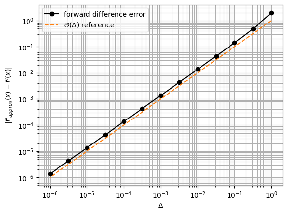
Exercise: Use the forward-difference approximation to approximate the derivative of \(e^x\) at \(x = 1\) for \(\Delta = 1\), \(0.1\), \(0.01\), and \(0.001\). Plot the absolute error as a function of \(\Delta\) using a log-log scale.
Solution:
[1]:
import numpy as np
import matplotlib.pyplot as plt

x = 1.0
dfdx_exact = np.exp(x)
Deltas = np.logspace(0, -6, 13)
dfdx_approx = np.zeros(len(Deltas))

for i, Delta in enumerate(Deltas):
    dfdx_approx[i] = (np.exp(x + Delta) - np.exp(x)) / Delta

plt.loglog(Deltas, abs(dfdx_approx - dfdx_exact), 'k-o', label='forward difference error')
plt.loglog(Deltas, Deltas, 'C1--', label=r'$\mathcal{O}(\Delta)$ reference')
plt.xlabel(r'$\Delta$')
plt.ylabel(r"$|f'_{approx}(x)-f'(x)|$")
plt.grid(True, which='both')
plt.legend();
Exercise: Repeat the previous exercise but use the backward difference. Do you observe any difference?
Back to Order
The solved exercise above suggests that the forward-difference approximation yields a better approximation as \(\Delta\) grows smaller, but how much better? To answer this, we consider the Taylor series for \(f(x+\Delta)\) about the point \(x\):
By isolating \(f'(x)\) on one side, we have
In other words, the forward difference leaves out terms proportional to \(\Delta\) and higher powers of \(\Delta\). Moreover, as \(\Delta\) shrinks, \(\Delta \gg \Delta^p\) for \(p > 1\). The terms left out represent the truncation error, and because this error goes as \(\Delta^1\) for small \(\Delta\), the order of the error is 1, i.e., the forward-difference approximation is a first-order approximation.
Exercise: Show that the backward-difference approximation is also first order.
Can we do better than first order? It turns out that we can. Consider the following Taylor series:
Subtraction of this series from the one above for \(f(x+\Delta)\) leads to
or
This latter approximation for \(f'(x)\) is a central difference and is a second-order approximation because \(\Delta\) is raised to the second power.
Note: Forward and backward differences yield first-order approximations to \(f'(x)\), while the central difference yields a second-order approximation for \(f'(x)\).
Exercise: Consider the Taylor series for \(f(x-\Delta)\), \(f(x+\Delta)\), \(f(x-2\Delta)\), and \(f(x+2\Delta)\). Try to develop a fourth-order approximation for \(f'(x)\) that involves these four values of \(f\).
Exercise: Consider a function \(f(x)\) for which you are given values only at \(x = i\Delta\) for \(i = 0, 1, 2, \ldots\) for small \(\Delta\). Suppose that some application requires that you evaluate \(f(x)\) at some middle point \((i+1/2)\Delta\). Of course, the natural thing to do is average the two adjacent values at \(i\Delta\) and \((i+1)\Delta\). What order is this averaging approximation?
Exercise: Apply the central difference to the function \(f(x) = \sin(2x - 0.17) + 0.3 \cos(3.4x + 0.1)\) at \(x = 0.5\). Plot the error for \(\Delta = 10^{-1}, 10^{-2}, \ldots, 10^{-7}\).
When Smaller Is Not Always Better
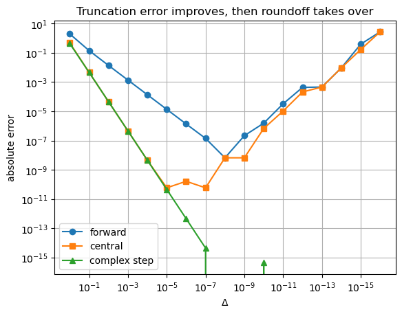
The Taylor-series argument says smaller \(\Delta\) should reduce truncation error. Floating-point arithmetic adds another effect: roundoff error. If \(f(x+\Delta)\) and \(f(x)\) are nearly equal, the subtraction can cancel many shared digits before division by \(\Delta\) amplifies the remaining noise.
For a smooth real function that can also accept complex inputs, the complex-step derivative approximation avoids that subtractive cancellation:
Why does this work? Taylor expand into the complex plane:
The imaginary part is \(\Delta f'(x) + \mathcal{O}(\Delta^3)\), so dividing by \(\Delta\) gives a second-order derivative estimate without subtracting two nearly equal real numbers.
Use this method for analytic callable functions that support complex inputs. Do not use it for already-sampled data, functions with non-analytic operations such as abs, or code paths that reject complex numbers.
[2]:
def forward_difference(f, x, Delta):
    return (f(x + Delta) - f(x)) / Delta


def central_difference(f, x, Delta):
    return (f(x + Delta) - f(x - Delta)) / (2 * Delta)


def complex_step_difference(f, x, Delta):
    return np.imag(f(x + 1j * Delta)) / Delta


def f(x):
    return np.exp(x)

x = 1.0
dfdx_exact = np.exp(x)
Deltas = np.logspace(0, -16, 17)

error_forward = np.array([abs(forward_difference(f, x, Delta) - dfdx_exact) for Delta in Deltas])
error_central = np.array([abs(central_difference(f, x, Delta) - dfdx_exact) for Delta in Deltas])
error_complex = np.array([abs(complex_step_difference(f, x, Delta) - dfdx_exact) for Delta in Deltas])

plt.loglog(Deltas, error_forward, 'o-', label='forward')
plt.loglog(Deltas, error_central, 's-', label='central')
plt.loglog(Deltas, error_complex, '^-', label='complex step')
plt.gca().invert_xaxis()
plt.xlabel(r'$\Delta$')
plt.ylabel('absolute error')
plt.grid(True, which='both')
plt.legend()
plt.title('Truncation error improves, then roundoff takes over');
Approximating the Second Derivative
So far, the finite differences developed represent approximations to the first derivative, \(f'(x)\). Approximations for the second derivative can be derived in a similar fashion. Consider again the Taylor series for \(f(x+\Delta)\) and \(f(x-\Delta)\). Whereas these series were subtracted to yield the central-difference approximation for \(f'(x)\), they can instead be added to yield the following:
where both the \(f'\) and \(f'''\) terms cancel. By isolating \(f''(x)\), we have
which is the central-difference approximation for the second derivative. Like the central-difference approximation for the first derivative, the truncation error is second order.
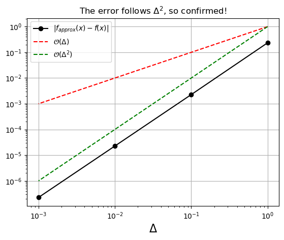
How can we establish order of accuracy? Earlier computational experiments used plots to reveal a trend; the same habit works here. Although order of accuracy is not the same thing as algorithmic complexity, the technique is similar: we test the approximation for different values of \(\Delta\) and see whether the error goes as \(\Delta\) or \(\Delta^2\) or something else entirely. By “see”, I mean literally: use a graphic!
Exercise: Confirm graphically that the central-difference approximation for the second derivative is, in fact, second order. Use \(f(x) = e^x\) for demonstration.
Solution: I set us up for success with the last solved exercise, which is adapted here.
[3]:
import numpy as np
import matplotlib.pyplot as plt
x = 1.0
fpp_ref = np.exp(x) # fpp for "f prime prime"
Delta = np.logspace(0, -3, 4)
d2fdx2_approx = np.zeros(len(Delta))
for i in range(len(Delta)):
    d2fdx2_approx[i] = (np.exp(x+Delta[i])-2*np.exp(x)+np.exp(x-Delta[i]))/Delta[i]**2
plt.loglog(Delta, abs(d2fdx2_approx-fpp_ref), 'k-o', label='$|f''_{approx}(x)-f''(x)|$')
plt.loglog(Delta, Delta, 'r--', label='$\mathcal{O}(\Delta)$')
plt.loglog(Delta, Delta**2, 'g--', label='$\mathcal{O}(\Delta^2)$')
plt.xlabel('$\Delta$', fontsize=16)
plt.legend()
plt.grid(True)
plt.title('The error follows $\Delta^2$, so confirmed!')
plt.show()
<>:10: SyntaxWarning: invalid escape sequence '\m'
<>:11: SyntaxWarning: invalid escape sequence '\m'
<>:12: SyntaxWarning: invalid escape sequence '\D'
<>:15: SyntaxWarning: invalid escape sequence '\D'
<>:10: SyntaxWarning: invalid escape sequence '\m'
<>:11: SyntaxWarning: invalid escape sequence '\m'
<>:12: SyntaxWarning: invalid escape sequence '\D'
<>:15: SyntaxWarning: invalid escape sequence '\D'
/tmp/ipykernel_1101175/3659422081.py:10: SyntaxWarning: invalid escape sequence '\m'
  plt.loglog(Delta, Delta, 'r--', label='$\mathcal{O}(\Delta)$')
/tmp/ipykernel_1101175/3659422081.py:11: SyntaxWarning: invalid escape sequence '\m'
  plt.loglog(Delta, Delta**2, 'g--', label='$\mathcal{O}(\Delta^2)$')
/tmp/ipykernel_1101175/3659422081.py:12: SyntaxWarning: invalid escape sequence '\D'
  plt.xlabel('$\Delta$', fontsize=16)
/tmp/ipykernel_1101175/3659422081.py:15: SyntaxWarning: invalid escape sequence '\D'
  plt.title('The error follows $\Delta^2$, so confirmed!')
From Derivatives to Gradients
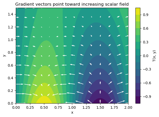
A one-dimensional derivative measures how a scalar function changes as one coordinate changes. For a scalar field \(T(x,y)\), the derivative information becomes a gradient:
The gradient points in the direction of steepest increase. Its components are partial derivatives: change \(x\) while holding \(y\) fixed, and change \(y\) while holding \(x\) fixed.
For sampled data on a grid, NumPy’s np.gradient applies finite-difference ideas along each array axis. The array convention matters: for a mesh built by X, Y = np.meshgrid(x, y), the field T has rows in the \(y\) direction and columns in the \(x\) direction, so
dTdy, dTdx = np.gradient(T, y, x, edge_order=2)
returns the \(y\) derivative first and the \(x\) derivative second.
[4]:
def temperature_field(x, y):
    return np.sin(np.pi * x) * np.exp(-y) + 0.15 * x * y


def exact_dTdx(x, y):
    return np.pi * np.cos(np.pi * x) * np.exp(-y) + 0.15 * y


def exact_dTdy(x, y):
    return -np.sin(np.pi * x) * np.exp(-y) + 0.15 * x

x = np.linspace(0.0, 2.0, 81)
y = np.linspace(0.0, 1.5, 61)
X, Y = np.meshgrid(x, y)
T = temperature_field(X, Y)

dTdy, dTdx = np.gradient(T, y, x, edge_order=2)

# Compare at an interior grid point.
j, i = 30, 40
print('sample point:', X[j, i], Y[j, i])
print('np.gradient dT/dx:', dTdx[j, i], 'exact:', exact_dTdx(X[j, i], Y[j, i]))
print('np.gradient dT/dy:', dTdy[j, i], 'exact:', exact_dTdy(X[j, i], Y[j, i]))

skip = (slice(None, None, 6), slice(None, None, 6))
plt.figure(figsize=(7, 4.8))
contours = plt.contourf(X, Y, T, levels=18, cmap='viridis')
plt.colorbar(contours, label='T(x, y)')
plt.quiver(X[skip], Y[skip], dTdx[skip], dTdy[skip], color='white', scale=35, width=0.004)
plt.xlabel('x')
plt.ylabel('y')
plt.title('Gradient vectors point toward increasing scalar field');
sample point: 1.0 0.75
np.gradient dT/dx: -1.3699581032055743 exact: -1.3714832918927073
np.gradient dT/dy: 0.15000000000000036 exact: 0.14999999999999994
Optional Extension: Higher-Order Stencils
The finite-difference approximations explored were identified pretty easily by manipulating the Taylor series of a function. Approximations that are higher order or that can be used for higher derivatives are somewhat more challenging to develop.
Simple Rules
Generally, approximations that use values of \(f\) at more values of \(x\) (e.g., \(x-\Delta\) and \(x+\Delta\)) are better than those that use fewer.
A more specific rule-of-thumb: an \(n\)th-order approximation for the \(m\)th derivative requires that \(f\) be evaluated at \(n+m-1\) evenly-spaced \(x\) values if those values are symmetric about \(x\) (e.g., \(x-\Delta\) and \(x+\Delta\) as used for the central difference) or \(n+m\) points, if the points are not symmetric about \(x\) (e.g., \(x-\Delta\) and \(x\) as used for the backward difference).
Exercise: Does the backward-difference approximation for \(df/dx\) follow this rule?
Solution: The backward-difference approximation for the first derivative (\(m=1\)) is first order (\(n=1\)). The points are not symmetric about \(x\). Hence, the rule requires \(m+n = 2\) points, consistent with the approximation.
Exercise: Does the forward-difference approximation for \(df/dx\) follow this rule?
Exercise: Does the central-difference approximation for \(df/dx\) follow this rule?
Exercise: Does the central-difference approximation for \(d^2f/dx^2\) follow this rule?
Further Reading
None for now.