Data Analysis via Interpolation

Overview, Objectives, and Key Terms

In Lesson 24, we treated measured data as

\[\mathbf{y} = \mathbf{A}\mathbf{x} + \boldsymbol{\epsilon},\]

where \(\mathbf{A}\) is the design matrix, \(\mathbf{x}\) contains model parameters, and \(\boldsymbol{\epsilon}\) is the measurement or modeling error. Least squares is natural when those deviations behave like samples of a zero-mean error process. With normal errors, the least-squares solution also has a statistical interpretation, and nonlinear models can be interpreted locally by linearizing around the best-fit parameters.

Interpolation answers a different question. It says: suppose the tabulated values are the model, at least at the tabulated points. How should we estimate values between them?

Objectives

By the end of this lesson, you should be able to

• interpret linear interpolation as a weighted sum,

• compute 1-D interpolation weights and connect them to np.interp,

• use CubicSpline when a smooth 1-D interpolant is appropriate,

• recognize regular grid interpolation as repeated 1-D interpolation,

• use RegularGridInterpolator for rectilinear 2-D and 3-D grid data,

• recognize unstructured interpolation as interpolation over triangles or tetrahedra,

• use LinearNDInterpolator for scattered points.

Key Terms

• interpolation

• extrapolation

• convex combination

• barycentric weights

• rectilinear grid

• triangulation

• np.interp

• CubicSpline

• RegularGridInterpolator

• LinearNDInterpolator

import numpy as np
import matplotlib.pyplot as plt
from matplotlib.tri import Triangulation
from scipy.interpolate import CubicSpline, LinearNDInterpolator, RegularGridInterpolator

COLORS = {
    "ink": "#1f2937",
    "muted": "#64748b",
    "grid": "#e5e7eb",
    "panel": "#fafaf7",
    "purple": "#512888",
    "orange": "#D55E00",
    "blue": "#2563eb",
    "green": "#059669",
    "red": "#dc2626",
}

plt.rcParams.update({
    "figure.facecolor": "white",
    "axes.facecolor": COLORS["panel"],
    "axes.edgecolor": COLORS["muted"],
    "axes.labelcolor": COLORS["ink"],
    "axes.titlecolor": COLORS["ink"],
    "xtick.color": COLORS["ink"],
    "ytick.color": COLORS["ink"],
    "grid.color": COLORS["grid"],
    "font.size": 11,
})


def style_axes(ax):
    ax.grid(True, alpha=0.5)
    ax.spines["top"].set_visible(False)
    ax.spines["right"].set_visible(False)

The Teeter-Totter: Two Points, Two Weights

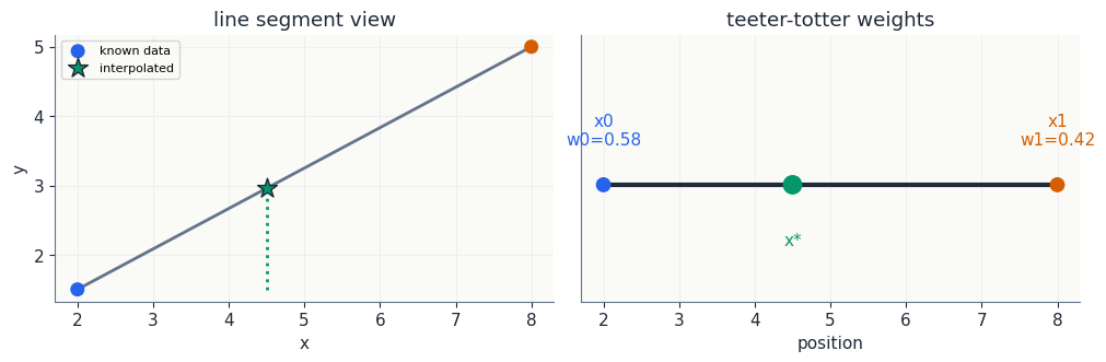
Start with two trusted points \((x_0,y_0)\) and \((x_1,y_1)\). We want the value at \(x_*\) between them. Instead of first writing a slope and intercept, write the interpolated value as a weighted sum:

\[y_* = w_0 y_0 + w_1 y_1.\]

The weights have two jobs. First, they must add to one:

\[w_0 + w_1 = 1.\]

Second, they must balance the horizontal location:

\[w_0 x_0 + w_1 x_1 = x_*.\]

Two equations, two unknowns. The solution is

\[w_0 = \frac{x_1-x_*}{x_1-x_0}, \qquad w_1 = \frac{x_*-x_0}{x_1-x_0}.\]

This is the teeter-totter picture: the point closer to \(x_*\) gets more weight.

x0, x1 = 2.0, 8.0
y0, y1 = 1.5, 5.0
x_star = 4.5
w0 = (x1 - x_star)/(x1 - x0)
w1 = (x_star - x0)/(x1 - x0)
y_star = w0*y0 + w1*y1

print("Input")
print(f"points: ({x0:.1f}, {y0:.1f}), ({x1:.1f}, {y1:.1f})")
print(f"target x*: {x_star:.1f}")
print("Output")
print(f"weights: w0={w0:.3f}, w1={w1:.3f}, sum={w0+w1:.3f}")
print(f"interpolated y*: {y_star:.3f}")

fig, axes = plt.subplots(1, 2, figsize=(10, 3.2), constrained_layout=True)
ax = axes[0]
ax.plot([x0, x1], [y0, y1], color=COLORS["muted"], lw=2)
ax.scatter([x0, x1], [y0, y1], color=[COLORS["blue"], COLORS["orange"]], s=70, zorder=3, label="known data")
ax.scatter([x_star], [y_star], marker="*", color=COLORS["green"], edgecolor=COLORS["ink"], s=180, zorder=4, label="interpolated")
ax.vlines(x_star, min(y0, y1), y_star, color=COLORS["green"], ls=":", lw=2)
ax.set_xlabel("x")
ax.set_ylabel("y")
ax.set_title("line segment view")
ax.legend(fontsize=8)
style_axes(ax)

ax = axes[1]
ax.hlines(0, x0, x1, color=COLORS["ink"], lw=3)
ax.scatter([x0, x1, x_star], [0, 0, 0], color=[COLORS["blue"], COLORS["orange"], COLORS["green"]], s=[80, 80, 140], zorder=3)
ax.text(x0, 0.12, f"x0\nw0={w0:.2f}", ha="center", color=COLORS["blue"])
ax.text(x1, 0.12, f"x1\nw1={w1:.2f}", ha="center", color=COLORS["orange"])
ax.text(x_star, -0.18, "x*", ha="center", color=COLORS["green"])
ax.set_ylim(-0.35, 0.45)
ax.set_yticks([])
ax.set_xlabel("position")
ax.set_title("teeter-totter weights")
style_axes(ax)
plt.show()

Input
points: (2.0, 1.5), (8.0, 5.0)
target x*: 4.5
Output
weights: w0=0.583, w1=0.417, sum=1.000
interpolated y*: 2.958

The 1-D Tool: np.interp

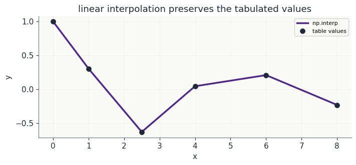
For 1-D linear interpolation, np.interp is the right first tool. It implements exactly the weighted-sum idea above, interval by interval.

Use it when:

• the data are 1-D,

• the \(x\) values are ordered,

• linear segments are appropriate,

• you want a simple, dependable interpolation rather than a fitted model.

# Input: a small table sampled from a smooth function.
x = np.array([0.0, 1.0, 2.5, 4.0, 6.0, 8.0])
y = np.exp(-0.18*x)*np.cos(1.2*x)
x_eval = np.linspace(x[0], x[-1], 300)

# Tool: 1-D linear interpolation.
y_linear = np.interp(x_eval, x, y)

print("Input")
print(f"number of table points: {len(x)}")
print(f"evaluation points     : {len(x_eval)}")
print("Output")
print(f"linear interpolation at x=3.0: {np.interp(3.0, x, y): .4f}")

fig, ax = plt.subplots(figsize=(7, 3.2), constrained_layout=True)
ax.plot(x_eval, y_linear, color=COLORS["purple"], lw=2.5, label="np.interp")
ax.scatter(x, y, color=COLORS["ink"], s=45, zorder=3, label="table values")
ax.set_xlabel("x")
ax.set_ylabel("y")
ax.set_title("linear interpolation preserves the tabulated values")
ax.legend(fontsize=8)
style_axes(ax)
plt.show()

Input
number of table points: 6
evaluation points     : 300
Output
linear interpolation at x=3.0: -0.4066

Smooth 1-D Interpolation: CubicSpline

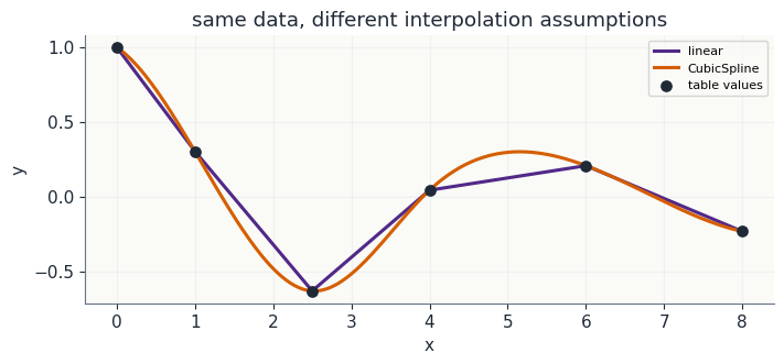
Sometimes straight segments are too angular for the task. A cubic spline still interpolates the data exactly, but it uses piecewise cubic polynomials with smooth connections between intervals.

That is not automatically better. A smoother curve is a stronger assumption. If the table is monotone and overshoot would be physically awkward, a shape-preserving tool such as PchipInterpolator is often preferable. The main point is to choose the tool that matches what you believe about the data.

# Tool: smooth 1-D interpolation.
spline = CubicSpline(x, y)
y_cubic = spline(x_eval)

fig, ax = plt.subplots(figsize=(7, 3.2), constrained_layout=True)
ax.plot(x_eval, y_linear, color=COLORS["purple"], lw=2.2, label="linear")
ax.plot(x_eval, y_cubic, color=COLORS["orange"], lw=2.2, label="CubicSpline")
ax.scatter(x, y, color=COLORS["ink"], s=45, zorder=3, label="table values")
ax.set_xlabel("x")
ax.set_ylabel("y")
ax.set_title("same data, different interpolation assumptions")
ax.legend(fontsize=8)
style_axes(ax)
plt.show()

Regular Grids: Repeat the Same Idea

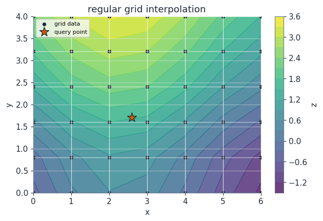
On a rectangular or rectilinear grid, 2-D linear interpolation is naturally sequential 1-D interpolation.

For a point inside one grid cell:

1. interpolate in \(x\) along the lower row,

2. interpolate in \(x\) along the upper row,

3. interpolate those two intermediate values in \(y\).

In 3-D, repeat the same idea one more time. This is why the modern SciPy tool is named RegularGridInterpolator: it works for 1-D, 2-D, 3-D, and higher-dimensional rectilinear grids.

def response(x, y):
    return np.sin(0.7*x) + 0.15*y**2 - 0.4*np.cos(1.2*y)

xg = np.linspace(0.0, 6.0, 7)
yg = np.linspace(0.0, 4.0, 6)
Xg, Yg = np.meshgrid(xg, yg, indexing="ij")
Zg = response(Xg, Yg)
point = np.array([2.6, 1.7])

# Manual sequential interpolation inside the containing cell.
ix = np.searchsorted(xg, point[0]) - 1
iy = np.searchsorted(yg, point[1]) - 1
x_left, x_right = xg[ix], xg[ix+1]
y_low, y_high = yg[iy], yg[iy+1]

z_low = np.interp(point[0], [x_left, x_right], [Zg[ix, iy], Zg[ix+1, iy]])
z_high = np.interp(point[0], [x_left, x_right], [Zg[ix, iy+1], Zg[ix+1, iy+1]])
z_manual = np.interp(point[1], [y_low, y_high], [z_low, z_high])

# Tool: regular-grid interpolation. Values have shape (len(xg), len(yg)).
rgi = RegularGridInterpolator((xg, yg), Zg, method="linear")
z_tool = float(rgi([point])[0])

print("Input")
print(f"grid shape: {Zg.shape}")
print(f"target point: ({point[0]:.2f}, {point[1]:.2f})")
print("Output")
print(f"manual sequential interpolation: {z_manual:.6f}")
print(f"RegularGridInterpolator       : {z_tool:.6f}")

fig, ax = plt.subplots(figsize=(6.2, 4.2), constrained_layout=True)
levels = ax.contourf(Xg, Yg, Zg, levels=16, cmap="viridis", alpha=0.78)
ax.plot(Xg, Yg, color="white", lw=0.8, alpha=0.65)
ax.plot(Xg.T, Yg.T, color="white", lw=0.8, alpha=0.65)
ax.scatter(Xg, Yg, s=18, color=COLORS["ink"], label="grid data")
ax.scatter([point[0]], [point[1]], marker="*", s=180, color=COLORS["orange"], edgecolor=COLORS["ink"], label="query point")
ax.set_xlabel("x")
ax.set_ylabel("y")
ax.set_title("regular grid interpolation")
ax.legend(fontsize=8, loc="upper left")
fig.colorbar(levels, ax=ax, label="z")
style_axes(ax)
plt.show()

Input
grid shape: (7, 6)
target point: (2.60, 1.70)
Output
manual sequential interpolation: 1.524157
RegularGridInterpolator       : 1.524157

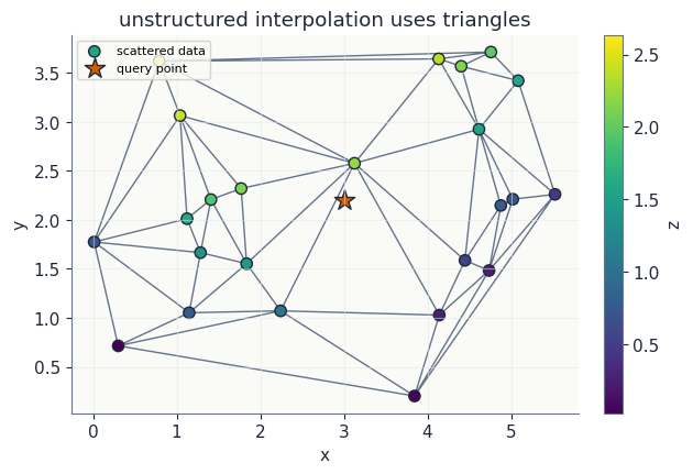
Unstructured Points: Barycentric Weights

Not all data arrive on a grid. In 2-D, scattered points can be triangulated. Inside one triangle, linear interpolation is still a weighted sum:

\[z_* = w_0 z_0 + w_1 z_1 + w_2 z_2,\]

with

\[w_0 + w_1 + w_2 = 1.\]

The extra equations make the weighted average land at the query point in both \(x\) and \(y\). These are barycentric weights. In 3-D, the same idea uses tetrahedra and four weights.

The matching SciPy tool for piecewise-linear interpolation on scattered points is LinearNDInterpolator. In 2-D, it triangulates the points; in 3-D, it uses tetrahedra.

rng = np.random.default_rng(415)
points = rng.random((24, 2))
points[:, 0] *= 6.0
points[:, 1] *= 4.0
values = response(points[:, 0], points[:, 1])
query = np.array([3.0, 2.2])

# Tool: scattered-data interpolation by triangulation.
scattered_interp = LinearNDInterpolator(points, values)
z_query = float(scattered_interp([query])[0])
tri = Triangulation(points[:, 0], points[:, 1])

print("Input")
print(f"scattered points: {len(points)}")
print(f"query point     : ({query[0]:.2f}, {query[1]:.2f})")
print("Output")
print(f"LinearNDInterpolator value: {z_query:.6f}")

fig, ax = plt.subplots(figsize=(6.2, 4.2), constrained_layout=True)
ax.triplot(tri, color=COLORS["muted"], lw=1.0)
sc = ax.scatter(points[:, 0], points[:, 1], c=values, cmap="viridis", s=55, edgecolor=COLORS["ink"], label="scattered data")
ax.scatter([query[0]], [query[1]], marker="*", s=190, color=COLORS["orange"], edgecolor=COLORS["ink"], label="query point")
ax.set_xlabel("x")
ax.set_ylabel("y")
ax.set_title("unstructured interpolation uses triangles")
ax.legend(fontsize=8, loc="upper left")
fig.colorbar(sc, ax=ax, label="z")
style_axes(ax)
plt.show()

Input
scattered points: 24
query point     : (3.00, 2.20)
Output
LinearNDInterpolator value: 1.885130

Tool Choice

A useful decision rule is:

• 1-D table, linear segments: use np.interp.

• 1-D table, smooth curve: use CubicSpline or a shape-preserving spline such as PchipInterpolator.

• 2-D, 3-D, or higher rectilinear grid: use RegularGridInterpolator.

• Unstructured 2-D or 3-D points: use LinearNDInterpolator for piecewise-linear interpolation.

• Old ``interp2d`` code: do not copy it into new work. It has been removed from SciPy; use RegularGridInterpolator for regular grids and scattered-data interpolators for unstructured points.

Interpolation is not fitting. It passes through the data. That is a feature when the table is the model, and a liability when the table is noisy.

Further Reading

• SciPy, interp2d transition guide

• SciPy, RegularGridInterpolator

• SciPy, LinearNDInterpolator

• SciPy, CubicSpline