Lesson 7 – Sampling Random Variables

Objectives

At the end of this lesson you should be able to

• Transform uniform random samples into samples from other distributions. In particular, derive and implement the inverse-transform method for the exponential distribution and compare your samples to NumPy’s built-in rng.exponential().

• Interpret histograms as empirical distributions. Use normalized histograms to assess whether a set of samples follows the intended distribution, and understand how bin width and sample size affect apparent noise.

• Modify the neutron simulation to use sampled flight distances. Replace the fixed step size \(\Delta x\) with exponentially distributed flight distances, and recognize how this change alters the physical model (mean free path and macroscopic cross section).

• Distinguish between parameters that change physics and those that change sampling noise. Recognize that increasing the number of neutrons reduces statistical uncertainty without changing the underlying probability, whereas changing step length or cross section changes the problem itself.

Lesson 06 described distributions. This lesson asks how to sample from them. We will start with uniform samples from rng.random(), transform them into exponential samples, and check the result with histograms. We will also return to the neutron walk and replace the artificial fixed step with a sampled flight distance.

Simulation modules and physical parameters

We begin by turning our neutron walk into a reusable module. In Python, a function such as run_simulation(c, n_steps, n_neutrons, seed) encapsulates the source–detector game so that we can import and reuse it in notebooks or slides. By varying its inputs we can explore how the detector response changes.

One key input is the number of steps (n_steps) used to traverse the distance to the detector. In Lesson 05 we used a fixed \(\Delta x\) and forced a collision after each step. Increasing the number of steps decreases \(\Delta x\) and increases the frequency of scattering events. This does not simply improve numerical accuracy; it changes the physical model by changing the mean free path. If we were modeling a slab of material, decreasing \(\Delta x\) is analogous to increasing the macroscopic cross section \(\Sigma\) (or attenuation coefficient \(\mu\)).

The fixed-step model can be summarized as

larger n_steps
    -> smaller Delta x
    -> more forced interaction opportunities
    -> more chances to reverse direction
    -> lower detector response

That last step is similar to the gambler’s ruin problem. A neutron that scatters many times has many chances to wander back through the left boundary before it ever reaches the detector. More steps do not merely make the calculation more accurate; they change the random walk that the neutron experiences.

In a physical transport model, interactions are not forced after a fixed step. Instead, the distance to the next interaction is random and is controlled by material data such as the macroscopic cross section \(\Sigma\).

Sampling the exponential distribution via inverse transform

To model free flights, we need to sample the distance a neutron travels before interacting. In a homogeneous medium, the flight distance \(S\) is an exponential random variable with PDF

\[f_S(s;\Sigma) = \Sigma e^{-\Sigma s},\quad s \geq 0\,.\]

Here \(\Sigma\) is the macroscopic cross section; its reciprocal \(1/\Sigma\) is the mean free path.

The inverse-transform method starts from a uniform sample \(U\sim\mathcal{U}(0,1)\) and uses the CDF of \(S\) to solve for \(S\) in terms of \(U\). The CDF of the exponential distribution is

\[F_S(s) = 1 - e^{-\Sigma s}\,.\]

Setting \(U = F_S(s)\) and solving for \(s\) gives

\[s = F_S^{-1}(U) = -\frac{1}{\Sigma} \ln(1 - U)\,.\]

Thus, to draw an exponential flight distance we can compute

import numpy as np
import matplotlib.pyplot as plt

Sigma = 2.0
rng = np.random.default_rng(12345)

u = rng.random()            # uniform on [0,1)
s = -np.log(1-u) / Sigma    # exponential sample

Here is a small implementation:

def sample_exponential_flight(Sigma, rng):
    u = rng.random()
    return -np.log(1.0 - u) / Sigma

The expression uses \(1-U\) instead of \(U\) to avoid the endpoint case \(\ln(0)\). Since \(U\) and \(1-U\) have the same uniform distribution on \([0,1)\), this does not change the distribution of the sampled distance.

NumPy already has an exponential sampler. Its scale parameter is the mean, so for \(f_S(s;\Sigma)=\Sigma e^{-\Sigma s}\) we use scale=1/Sigma:

Sigma = 2.0
rng = np.random.default_rng(12345)

s_manual = np.array([sample_exponential_flight(Sigma, rng) for _ in range(10_000)])
s_numpy = rng.exponential(scale=1/Sigma, size=10_000)

Empirical distributions and histograms

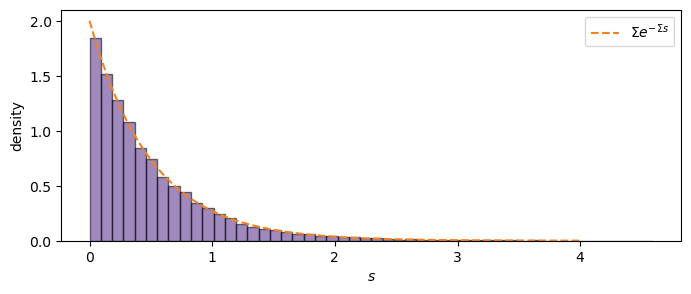
When we draw a finite number of samples from a distribution, we obtain an empirical distribution. A useful way to visualize an empirical distribution is with a histogram. In Python, calling plt.hist(samples, bins=n, density=True) divides the data into n bins and plots the fraction of samples in each bin.

Choosing the number of bins involves a trade-off: too few bins and important features are hidden; too many bins and the finite sample leads to noisy fluctuations. Normalizing the histogram (with density=True) turns counts into densities so that the area under the histogram approximates 1.

For the exponential distribution, we can compare sampled distances with the theoretical density:

purple = "#512888"
orange = "#F58220"

Sigma = 2.0
rng = np.random.default_rng(12345)
s = rng.exponential(scale=1/Sigma, size=10_000)

s_grid = np.linspace(0, 4, 400)
f_grid = Sigma*np.exp(-Sigma*s_grid)

plt.figure(figsize=(8, 3))
plt.hist(s, bins=50, density=True, color=purple, alpha=0.55, edgecolor="black")
plt.plot(s_grid, f_grid, color=orange, linestyle="--", label=r"$\Sigma e^{-\Sigma s}$")
plt.xlabel("$s$")
plt.ylabel("density")
plt.legend();

Changing the number of bins changes the appearance of the histogram:

plt.figure(figsize=(8, 3))
plt.hist(s, bins=500, density=True, color=purple, alpha=0.55, edgecolor="black")
plt.plot(s_grid, f_grid, color=orange, linestyle="--")
plt.xlabel("$s$")
plt.ylabel("density");

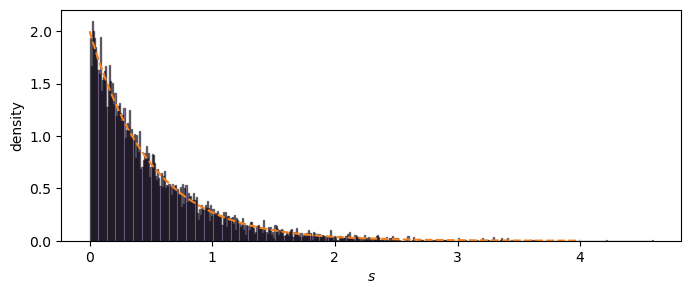
The second plot may look much noisier, even though it uses the same data. That noise is not a new physical effect. It is a finite-sample visualization effect caused by asking each bin to represent fewer samples.

Incorporating exponential flights into the neutron walk

With an exponential sampler in hand, we can revise the neutron simulation. Replace the fixed step size \(\Delta x\) with a flight distance sampled from \(\text{Exp}(\Sigma)\). For each neutron:

• Set its position to 0 and direction to \(+1\) or \(-1\).

• While the neutron is alive:

  • Draw \(s\sim\text{Exp}(\Sigma)\) and update the position: \(x \leftarrow x + s\,d\), where \(d\in\{+1,-1\}\) is the direction.

  • If \(x < 0\), the neutron escapes left; terminate the loop.

  • If \(x > L\), the neutron hits the detector; record a count and terminate the loop.

  • Otherwise, scatter: choose a new direction \(d\) uniformly from \(\{+1, -1\}\).

Because the exponential distribution has unbounded support, a rare neutron might take an extremely long flight. To prevent infinite loops in practice, impose a maximum collision count; if a neutron exceeds this limit, terminate the loop and treat it as escaped.

The modified history has the same overall structure as Lesson 05. The key difference is the sampled flight distance:

start neutron at x = 0
choose initial direction
for collision in 1, 2, ..., max_collisions:
    sample flight distance s from Exp(Sigma)
    move x <- x + s*d
    if x < 0:
        return 0
    if x > L:
        return 1
    choose a new direction d
return 0

The final return 0 is a defensive programming choice. It prevents a rare or buggy history from running forever. When using such a guard, we should choose max_collisions large enough that it does not affect ordinary histories and then check whether changing it changes the estimated response.

Looking ahead

Having learned how to sample flight distances and inspect empirical distributions, we will next turn to statistics and estimators. In Lesson 08 we will interpret the detector response as a Bernoulli random variable, compute its mean and variance, and study how repeated simulations lead to distributions of estimates. We will also introduce the normal approximation and the concept of standard error.

Sampling is not the final goal. Sampling is how we generate histories. The engineering quantity is still an estimate of a physical response, such as the probability that a source neutron reaches a detector. Lesson 08 asks how much that estimate should wiggle from run to run and how to report the uncertainty responsibly.