Lesson 8 – Statistics and Estimators

In Lesson 05 we performed our first Monte Carlo simulation using only uniform random numbers, and in Lesson 06 we formalized these numbers as samples of random variables with well-defined distributions. Lesson 07 introduced the mechanics of sampling from non-uniform distributions and modified the neutron walk to use exponentially distributed flight distances. Now we turn to the statistics of Monte Carlo outputs themselves: how do we model the detector response, estimate its parameters, and quantify the uncertainty of our estimates?

Objectives

After completing this lesson you should be able to

• Model detector response as a Bernoulli random variable. Identify the hit/no-hit outcome for a single neutron as an instance of the Bernoulli distribution, and write down its probability mass function.

• Compute distributional mean and variance. Use the definition of expectation to derive the mean and variance for a Bernoulli random variable with parameter \(p\).

• Define and use estimators. Distinguish between statistics computed from data (sample mean \(\bar{X}\), sample variance \(s^2\)) and the corresponding population parameters (the true probability \(p\), the mean \(\mu\), the variance \(\sigma^2\)). Explain what it means for an estimator to be unbiased and consistent.

• Quantify uncertainty with the Central Limit Theorem and normal approximation. Describe how repeated Monte Carlo runs produce a distribution of estimates, and use the normal approximation and standard error to put an uncertainty band on \(\bar{X}\).

The new idea in this lesson is that a Monte Carlo answer is itself random. The model has a probability \(p\), but a finite simulation produces an estimate \(\hat{p}\). If we repeat the same simulation with a different random seed, the estimate usually changes. Statistics gives us language for describing that wiggle.

Revisiting the simulation

To set the stage, run the neutron simulation with a fixed number of neutrons and vary the number of steps. The function run_simulation(c, n_steps, n_neutrons, seed) returns the fraction of neutrons that reach the detector. For example:

from L08_StatisticsAndEstimators import run_simulation

for steps in range(1, 10):
    response = run_simulation(c=1.0, n_steps=steps, n_neutrons=1000, seed=1234)
    print(f"{steps} steps, response = {response:.4f}")

1 steps, response = 0.5020
2 steps, response = 0.3390
3 steps, response = 0.2620
4 steps, response = 0.1990
5 steps, response = 0.1780
6 steps, response = 0.1230
7 steps, response = 0.1160
8 steps, response = 0.1160
9 steps, response = 0.0970

This simple experiment provides concrete numbers to connect with the abstract concepts below.

There are two different effects to keep separate:

• Changing n_steps changes the physical random walk in this simplified model.

• Changing the random seed changes the finite sample used to estimate the response.

If you run the same case several times without fixing the seed, the response will not be identical each time:

for trial in range(5):
    response = run_simulation(c=1.0, n_steps=4, n_neutrons=1000)
    print(f"trial {trial}: response = {response:.4f}")

trial 0: response = 0.2220
trial 1: response = 0.1880
trial 2: response = 0.1850
trial 3: response = 0.2040
trial 4: response = 0.1660

That variation is not a bug. It is the statistical behavior we need to quantify.

Modeling the detector response

A single neutron either hits the detector (value 1) or misses (value 0). We denote this binary outcome by a random variable \(X\) that takes values in \(\{0, 1\}\). It is natural to model \(X\) as a Bernoulli random variable with parameter \(p\) equal to the probability of detection:

• \(P(X = 1) = p\)

• \(P(X = 0) = 1 - p\)

The expected value (mean) and variance of \(X\) follow directly from the definition of expectation:

• \(E[X] = 0(1-p) + 1p = p\)

• \(\operatorname{Var}(X) = p(1-p)\)

These are population or distributional quantities—we cannot observe them directly but can derive them from the model. Note that \(E[X]\) is commonly denoted by \(\mu\) and \(\operatorname{Var}(X)\) by \(\sigma^2\).

The variance derivation is short enough to do directly. Since \(E[X]=p\),

\[\operatorname{Var}(X)=E[(X-p)^2]\,.\]

For a Bernoulli random variable,

\[\operatorname{Var}(X)=(0-p)^2(1-p)+(1-p)^2p =p^2(1-p)+p(1-p)^2 =p(1-p)\,.\]

This result passes a useful sanity check. If \(p=0\) or \(p=1\), the outcome is certain and the variance is zero. If \(p=0.5\), the uncertainty is largest and the variance is \(0.25\).

Estimating the parameter \(p\)

In practice we do not know \(p\); we must estimate it from data. Suppose we run the simulation with \(N\) neutrons and record outcomes \(X_1, X_2, \ldots, X_N\). Any function of these observations is a statistic; a statistic used to infer \(p\) is an estimator. The most natural estimator for \(p\) is the sample mean

\[\hat{p} = \frac{X_1 + X_2 + \cdots + X_N}{N}\]

This estimator is unbiased (its expectation is equal to \(p\)) and consistent (it converges to \(p\) as \(N\) grows). More generally, for any distribution with mean \(\mu\), the sample mean is an unbiased estimator of \(\mu\).

The sample variance provides an estimator for the population variance \(\sigma^2\):

\[s^2 = \frac{(X_1-\hat{p})^2 + (X_2-\hat{p})^2 + \cdots + (X_N-\hat{p})^2}{N-1}\]

When \(N\) is large, \(s^2\) is a good approximation to \(\sigma^2\).

The vocabulary is worth being careful about:

• A statistic is any quantity computed from the observed data.

• An estimator is a statistic used to estimate an unknown model parameter.

• An estimate is the numerical value produced by an estimator for one dataset.

The sample mean is an unbiased estimator of \(p\) because

\[E[\hat{p}] =E\left[\frac{1}{N}\sum_{i=1}^N X_i\right] =\frac{1}{N}\sum_{i=1}^N E[X_i] =\frac{1}{N}\sum_{i=1}^N p =p\,.\]

So \(\hat{p}\) may wiggle from run to run, but it is centered on the model probability.

Sampling distributions and the Central Limit Theorem

Because each Monte Carlo run yields a random estimate \(\hat{p}\), the estimator itself is a random variable. The distribution of \(\hat{p}\) over repeated independent runs is called its sampling distribution. The Central Limit Theorem (CLT) tells us that when \(N\) is large and the \(X_i\) are independent with mean \(\mu\) and variance \(\sigma^2\), the sample mean is approximately normally distributed with mean \(\mu\) and variance \(\sigma^2/N\).

In the Bernoulli case, \(\sigma^2 = p(1-p)\). Since \(p\) is unknown, we substitute the sample variance \(s^2\) into the CLT. The standard error of the sample mean is then

\[\epsilon = \sqrt{\frac{s^2}{N}}\]

Approximately 68 % of the time the true mean \(\mu\) lies within \(\hat{p} \pm \epsilon\), and about 95 % of the time it lies within \(\hat{p} \pm 2\epsilon\).

The normal distribution is the familiar bell-shaped distribution. We write

\[Z\sim\mathcal{N}(\mu,\sigma^2)\]

for a normal random variable with mean \(\mu\) and variance \(\sigma^2\).

The Central Limit Theorem is not saying that the individual neutron outcomes become normal. Each neutron outcome is still 0 or 1. The theorem is about the sample mean. When \(N\) is large, repeated values of \(\hat{p}\) from repeated simulations tend to form an approximately normal cloud centered near \(p\).

For Bernoulli outcomes, the ideal standard error would be

\[\sqrt{\frac{p(1-p)}{N}}\,.\]

Since \(p\) is unknown in a real simulation, we estimate this with \(\sqrt{s^2/N}\).

Example: repeated simulations and a normal overlay

To visualize the sampling distribution of \(\hat{p}\), run the same neutron simulation many times and collect the responses:

from L08_StatisticsAndEstimators import run_simulation
import numpy as np
import matplotlib.pyplot as plt

purple = "#512888"
orange = "#F58220"

# collect 1000 estimates of p_hat with N=1000 neutrons per run
responses = [run_simulation(c=1.0, n_steps=4, n_neutrons=1000) for j in range(1000)]

plt.figure(figsize=(8, 3))
plt.hist(responses, bins=25, density=True, color=purple, edgecolor="black", alpha=0.55)
plt.xlabel(r"estimated detector response, $\hat{p}$")
plt.ylabel("density");

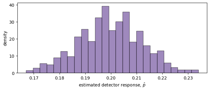
If the true detection probability is \(p=0.2\), the population mean and variance are \(\mu=0.2\) and \(\sigma^2=p(1-p)=0.16\). According to the CLT, the sample mean of \(N=1000\) Bernoulli trials is approximately normally distributed with variance \(\sigma^2/N = 0.16/1000\). Overlaying this normal approximation on the histogram shows how well it matches the empirical distribution:

x_vals = np.linspace(0.15, 0.25, 100)
norm_pdf = lambda x, a, b: 1/np.sqrt(2*np.pi*b) * np.exp(-(x-a)**2/(2*b))

plt.figure(figsize=(8, 3))
plt.hist(responses, bins=25, density=True, color=purple, edgecolor="black", alpha=0.55, label="sample means")
plt.plot(x_vals, norm_pdf(x_vals, 0.2, 0.16/1000), color=orange, linewidth=2, label=r"$\mathcal{N}(p, p(1-p)/N)$")
plt.xlabel(r"estimated detector response, $\hat{p}$")
plt.ylabel("density")
plt.legend();

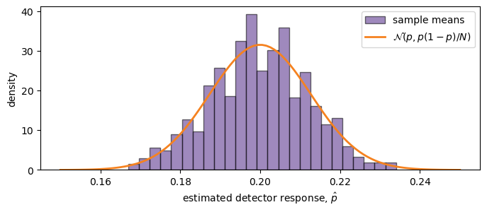
This overlay reveals the bell-shaped distribution of sample means centered near the true \(p\). The approximation improves as the number of neutrons \(N\) increases.

np.sqrt(0.16/1000)

np.float64(0.012649110640673518)

Try repeating the experiment with different values of n_neutrons:

for n_neutrons in [100, 1000, 10_000]:
    responses = [
        run_simulation(c=1.0, n_steps=4, n_neutrons=n_neutrons)
        for j in range(500)
    ]
    print(
        n_neutrons,
        np.mean(responses),
        np.std(responses, ddof=1),
        np.sqrt(0.2*(1-0.2)/n_neutrons),
    )

100 0.20088 0.04044375098810663 0.04
1000 0.200922 0.01241160795481585 0.01264911064067352
10000 0.200191 0.0041205894620830715 0.004

The last two numbers compare the observed spread of repeated estimates with the CLT prediction. As \(N\) increases, the histogram of estimates should become narrower, and the standard error should scale like \(1/\sqrt{N}\).

Summary and looking forward

In this lesson we modeled the detector response as a Bernoulli random variable, derived its mean and variance, and introduced the concepts of estimators, sample mean, and sample variance. We saw that the sample mean is an unbiased and consistent estimator of the true detection probability \(p\). By invoking the Central Limit Theorem and the normal distribution, we learned how to quantify the uncertainty in our Monte Carlo estimates using the standard error. These statistical tools will appear throughout the remainder of the course whenever we assess the reliability of Monte Carlo results.

This closes the first Monte Carlo probability block, but the ideas will keep appearing. Whenever we compute a response from sampled histories, we should ask three questions:

1. What model quantity are we estimating?

2. What statistic are we using as the estimator?

3. How much sampling uncertainty remains in the estimate?

Those questions matter for detector response, shielding calculations, criticality estimates, cross-section processing, and any other calculation where random histories are used to estimate a physical observable.