Solving ODEs Symbolically
Overview, Objectives, and Key Terms
L26 gave us a family of balance laws. Some balances stayed algebraic. Some reduced to ordinary differential equations. Some stayed as partial differential equations until we made one more assumption.
Today the organizing idea is simple:
reduce the balance to algebra when you can, then solve and check the result.
SymPy is useful here because it lets us keep parameters visible. A numerical solver can tell us one answer for one set of numbers. A symbolic expression can show the time scale, the equilibrium value, the boundary influence, or the mode that controls the physics.
By the end of this lesson, you should be able to:
define SymPy symbols and functions without confusing them,
solve simple linear IVPs and BVPs with
dsolve,apply initial and boundary data to symbolic constants,
check a symbolic solution by substitution,
use an ansatz to turn a differential equation into algebra,
recognize separation of variables as a symbolic reduction of a PDE.
Key terms. symbolic function, initial value problem, boundary value problem, ansatz, characteristic equation, separation of variables, eigenvalue, mode, residual.
[ ]:
import numpy as np
import sympy as sy
import matplotlib.pyplot as plt

sy.init_printing()

COLORS = {
    "ink": "#1f2937",
    "muted": "#64748b",
    "grid": "#cbd5e1",
    "panel": "#f8fafc",
    "purple": "#512888",
    "orange": "#D55E00",
    "blue": "#2563eb",
    "green": "#059669",
    "red": "#dc2626",
}

def style_axes(ax):
    ax.spines["top"].set_visible(False)
    ax.spines["right"].set_visible(False)
    ax.spines["left"].set_color(COLORS["muted"])
    ax.spines["bottom"].set_color(COLORS["muted"])
    ax.tick_params(colors=COLORS["muted"])
    ax.xaxis.label.set_color(COLORS["ink"])
    ax.yaxis.label.set_color(COLORS["ink"])
    ax.title.set_color(COLORS["ink"])
    ax.grid(True, color=COLORS["grid"], alpha=0.45, linewidth=0.7)
From L26 to L27
The one-dimensional ADR balance from L26 was
Different assumptions give different symbolic problems:
Assumptions |
Reduced model |
What we solve |
|---|---|---|
no space, transient |
\(u'=-\Sigma u+s_0\) |
first-order IVP |
steady, no diffusion |
\(w u' + \Sigma u=s_0\) |
first-order ODE with inflow data |
steady, no advection |
\(-D u''+\Sigma u=s_0\) |
second-order BVP |
no source, no advection |
\(u_t=D u_{xx}-\Sigma u\) |
PDE, often separated into modes |
The trick is not to memorize a different solver for each row. The trick is to write the reduced balance clearly, state the data, and check the answer.
[ ]:
# Input: several L26 balances and their L27 symbolic form.
reductions = [
    ("well-mixed reaction", "u' = -Sigma*u + s0", "linear IVP"),
    ("steady 1-D flow", "w*u' + Sigma*u = s0", "inflow ODE"),
    ("steady slab diffusion", "-D*u'' + Sigma*u = s0", "two-point BVP"),
    ("modal diffusion-reaction", "u_t = D*u_xx - Sigma*u", "separation / eigenvalue"),
]

print("Input")
print("Each row starts from the L26 balance and adds assumptions.")
print("Output")
for name, model, kind in reductions:
    print(f"{name:27s} -> {model:27s} ({kind})")
Input
Each row starts from the L26 balance and adds assumptions.
Output
well-mixed reaction         -> u' = -Sigma*u + s0          (linear IVP)
steady 1-D flow             -> w*u' + Sigma*u = s0         (inflow ODE)
steady slab diffusion       -> -D*u'' + Sigma*u = s0       (two-point BVP)
modal diffusion-reaction    -> u_t = D*u_xx - Sigma*u      (separation / eigenvalue)
Symbols Are Not Functions
This is the most common SymPy mistake in this lesson. A symbol like t is an independent variable. A symbolic function like u(t) must be created with sy.Function.
Use this pattern:
t = sy.symbols("t")
u = sy.Function("u")
u(t)
Do not create u with sy.symbols and then try to call u(t). A symbol is not callable.
[ ]:
# Input: independent variable and unknown symbolic function.
t = sy.symbols("t", real=True)
u = sy.Function("u")

print("Input")
print(f"t is a {type(t).__name__}")
print(f"u is a {type(u).__name__}")
print("Output")
print("The symbolic unknown is u(t):")
u(t)
Input
t is a Symbol
u is a UndefinedFunction
Output
The symbolic unknown is u(t):
A Reusable Symbolic Scaffold
For the rest of your ODE-solving career, a safe symbolic workflow is:
define the independent variable and unknown function,
write the differential equation as
sy.Eq(left, right),solve with
sy.dsolveor solve for constants by hand,check the solution by substitution,
turn the expression into a numerical function with
sy.lambdifywhen you want values or plots.
The checking step matters. It catches sign errors, missing constants, and boundary conditions that were not actually applied.
Example 1: Pure Reaction with a Constant Source
Start with the L26 reduction for a well-mixed amount or density:
This is the balance statement
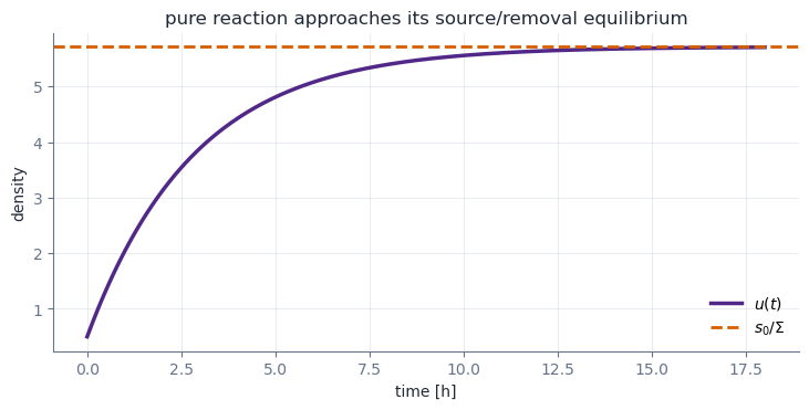
The equilibrium value should be \(u=s_0/\Sigma\). The symbolic solution should make that visible.
[ ]:
# Input block: symbols, unknown function, and pure reaction balance.
t = sy.symbols("t", real=True)
Sigma, s0, u0 = sy.symbols("Sigma s_0 u_0", positive=True)
u = sy.Function("u")

reaction_ode = sy.Eq(sy.diff(u(t), t), -Sigma*u(t) + s0)
reaction_solution = sy.dsolve(reaction_ode, ics={u(0): u0})
u_reaction = sy.simplify(reaction_solution.rhs)

reaction_residual = sy.simplify(sy.diff(u_reaction, t) + Sigma*u_reaction - s0)
initial_residual = sy.simplify(u_reaction.subs(t, 0) - u0)

equilibrium = sy.simplify(sy.limit(u_reaction, t, sy.oo))

print("Input")
print("du/dt = -Sigma*u + s0, u(0)=u0")
print("Output")
print(f"ODE residual      : {reaction_residual}")
print(f"initial residual  : {initial_residual}")
print(f"long-time value   : {equilibrium}")
u_reaction
Input
du/dt = -Sigma*u + s0, u(0)=u0
Output
ODE residual      : 0
initial residual  : 0
long-time value   : s_0/Sigma
[ ]:
# Input block: numerical values for the symbolic reaction solution.
reaction_values = {
    Sigma: 0.35,   # 1/h
    s0: 2.0,       # density/h
    u0: 0.5,       # initial density
}

tu = np.linspace(0.0, 18.0, 250)
u_fun = sy.lambdify((t, Sigma, s0, u0), u_reaction, "numpy")
u_vals = u_fun(tu, reaction_values[Sigma], reaction_values[s0], reaction_values[u0])
ueq = float(equilibrium.subs(reaction_values))

print("Input")
for key, value in reaction_values.items():
    print(f"{key}: {value}")
print("Output")
print(f"equilibrium density: {ueq:.3f}")
print(f"u(18 h): {u_vals[-1]:.3f}")

fig, ax = plt.subplots(figsize=(7.2, 3.6), constrained_layout=True)
ax.plot(tu, u_vals, color=COLORS["purple"], lw=2.5, label="$u(t)$")
ax.axhline(ueq, color=COLORS["orange"], ls="--", lw=2, label="$s_0/\\Sigma$")
ax.set_xlabel("time [h]")
ax.set_ylabel("density")
ax.set_title("pure reaction approaches its source/removal equilibrium")
ax.legend(frameon=False)
style_axes(ax)
plt.show()
Input
Sigma: 0.35
s_0: 2.0
u_0: 0.5
Output
equilibrium density: 5.714
u(18 h): 5.705
Example 2: Steady Advection-Reaction in a Flow
Now keep one spatial coordinate, but make the problem steady and neglect diffusion:
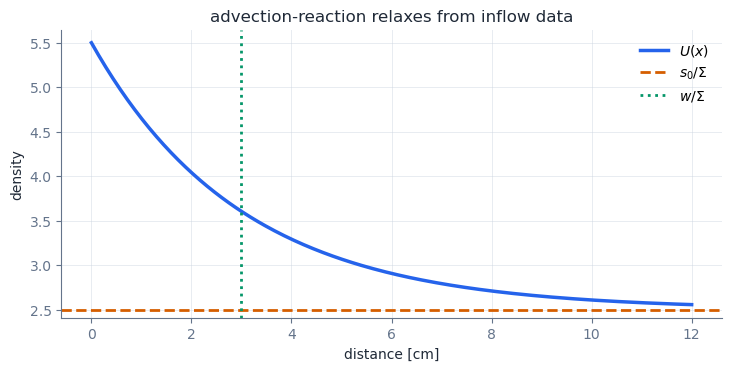
This is the same source-removal balance, but the independent variable is now distance. The inflow value replaces the initial value. The symbolic solution should relax toward \(s_0/\Sigma\) over a length scale \(w/\Sigma\).
[ ]:
# Input block: steady advection-reaction balance.
x = sy.symbols("x", real=True)
w, Sigma_x, s0_x, u_in = sy.symbols("w Sigma s_0 u_in", positive=True)
U = sy.Function("U")

adv_reaction_ode = sy.Eq(w*sy.diff(U(x), x) + Sigma_x*U(x), s0_x)
adv_reaction_solution = sy.dsolve(adv_reaction_ode, ics={U(0): u_in})
u_adv = sy.simplify(adv_reaction_solution.rhs)

adv_residual = sy.simplify(w*sy.diff(u_adv, x) + Sigma_x*u_adv - s0_x)
inflow_residual = sy.simplify(u_adv.subs(x, 0) - u_in)
length_scale = sy.simplify(w/Sigma_x)

print("Input")
print("w*dU/dx + Sigma*U = s0, U(0)=u_in")
print("Output")
print(f"ODE residual     : {adv_residual}")
print(f"inflow residual  : {inflow_residual}")
print(f"length scale     : {length_scale}")
u_adv
Input
w*dU/dx + Sigma*U = s0, U(0)=u_in
Output
ODE residual     : 0
inflow residual  : 0
length scale     : w/Sigma
[ ]:
# Input block: numerical values for the spatial balance.
adv_values = {
    w: 1.2,          # cm/s
    Sigma_x: 0.4,    # 1/s
    s0_x: 1.0,       # density/s
    u_in: 5.5,       # inflow density
}

xx = np.linspace(0.0, 12.0, 250)
adv_fun = sy.lambdify((x, w, Sigma_x, s0_x, u_in), u_adv, "numpy")
adv_vals = adv_fun(xx, adv_values[w], adv_values[Sigma_x], adv_values[s0_x], adv_values[u_in])
adv_eq = float((s0_x/Sigma_x).subs(adv_values))
ell = float(length_scale.subs(adv_values))

print("Input")
for key, value in adv_values.items():
    print(f"{key}: {value}")
print("Output")
print(f"equilibrium density: {adv_eq:.3f}")
print(f"relaxation length  : {ell:.3f} cm")
print(f"U(12 cm): {adv_vals[-1]:.3f}")

fig, ax = plt.subplots(figsize=(7.2, 3.6), constrained_layout=True)
ax.plot(xx, adv_vals, color=COLORS["blue"], lw=2.5, label="$U(x)$")
ax.axhline(adv_eq, color=COLORS["orange"], ls="--", lw=2, label="$s_0/\\Sigma$")
ax.axvline(ell, color=COLORS["green"], ls=":", lw=2, label="$w/\\Sigma$")
ax.set_xlabel("distance [cm]")
ax.set_ylabel("density")
ax.set_title("advection-reaction relaxes from inflow data")
ax.legend(frameon=False)
style_axes(ax)
plt.show()
Input
w: 1.2
Sigma: 0.4
s_0: 1.0
u_in: 5.5
Output
equilibrium density: 2.500
relaxation length  : 3.000 cm
U(12 cm): 2.555
Ansatz: Guess a Shape, Reduce to Algebra
An ansatz is an assumed solution shape. The point is not guessing randomly. The point is choosing a shape that derivatives reproduce.
For a constant-coefficient homogeneous ODE,
the exponential trial function \(y=e^{rt}\) turns differentiation into multiplication by \(r\). Substitution reduces the ODE to the characteristic equation
[ ]:
# Input block: characteristic-equation reduction.
r, a, b = sy.symbols("r a b")
y_trial = sy.exp(r*t)
char_residual = sy.simplify(sy.diff(y_trial, t, 2) + a*sy.diff(y_trial, t) + b*y_trial)
char_equation = sy.factor(char_residual / y_trial)
roots = sy.solve(sy.Eq(char_equation, 0), r)

print("Input")
print("trial solution y = exp(r*t)")
print("Output")
print(f"characteristic equation: {char_equation} = 0")
print(f"roots: {roots}")
Input
trial solution y = exp(r*t)
Output
characteristic equation: a*r + b + r**2 = 0
roots: [-a/2 - sqrt(a**2 - 4*b)/2, -a/2 + sqrt(a**2 - 4*b)/2]
PDE Example: Separation of Variables
The same idea helps with PDEs. Consider the source-free, one-dimensional reaction-diffusion model from L26:
Start with the simplest separable ansatz:
Substitute into the PDE and divide by \(T(t)X(x)\):
The left side depends only on \(t\). The right side depends only on \(x\). For one equality to hold for all \(x\) and \(t\), both sides must be the same constant. We choose the sign convention
Then
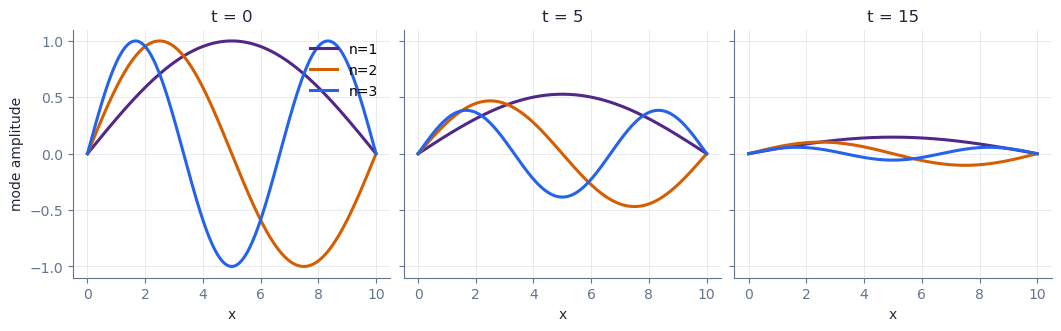
So \(\lambda\) is the decay rate for that separated mode. If \(\lambda>0\), the time constant is \(1/\lambda\). The spatial part becomes the eigenvalue problem
[ ]:
# Input block: start with a generic separated ansatz.
x, t = sy.symbols("x t", real=True)
D, Sigma, L, lam = sy.symbols("D Sigma L lambda", positive=True)
T = sy.Function("T")
X = sy.Function("X")

separable_ansatz = T(t) * X(x)
separation_residual = sy.simplify(
    sy.diff(separable_ansatz, t)
    - D*sy.diff(separable_ansatz, x, 2)
    + Sigma*separable_ansatz
)
separation_ratio = sy.simplify(separation_residual / separable_ansatz)
time_solution = sy.dsolve(sy.Eq(sy.diff(T(t), t), -lam*T(t)))

print("Input")
print("v(x,t) = T(t)*X(x)")
print("Output")
print(f"residual / (T*X): {separation_ratio}")
print(f"time equation solution: {time_solution}")
separation_ratio
Input
v(x,t) = T(t)*X(x)
Output
residual / (T*X): -D*Derivative(X(x), (x, 2))/X(x) + Sigma + Derivative(T(t), t)/T(t)
time equation solution: Eq(T(t), C1*exp(-lambda*t))
Boundary Conditions Select the Allowed Modes
For the zero-value boundary conditions \(v(0,t)=v(L,t)=0\), a compatible spatial shape is
Substitute the full mode
Now the PDE residual reduces to one algebraic expression for \(\lambda_n\).
[ ]:
# Input block: boundary-compatible separated reaction-diffusion mode.
n = sy.symbols("n", integer=True, positive=True)

v_mode = sy.exp(-lam*t) * sy.sin(n*sy.pi*x/L)
pde_residual = sy.simplify(sy.diff(v_mode, t) - D*sy.diff(v_mode, x, 2) + Sigma*v_mode)
mode_factor = sy.simplify(pde_residual / v_mode)
lam_n = sy.solve(sy.Eq(mode_factor, 0), lam)[0]

print("Input")
print("v_n(x,t) = exp(-lambda*t)*sin(n*pi*x/L)")
print("Output")
print(f"mode residual / mode: {mode_factor}")
print(f"lambda_n: {lam_n}")
lam_n
Input
v_n(x,t) = exp(-lambda*t)*sin(n*pi*x/L)
Output
mode residual / mode: pi**2*D*n**2/L**2 + Sigma - lambda
lambda_n: pi**2*D*n**2/L**2 + Sigma
[ ]:
# Input block: plot the first three separated modes.
mode_values = {D: 0.08, Sigma: 0.12, L: 10.0}
xgrid = np.linspace(0.0, mode_values[L], 300)
times = [0.0, 5.0, 15.0]
mode_numbers = [1, 2, 3]

print("Input")
print(f"D={mode_values[D]}, Sigma={mode_values[Sigma]}, L={mode_values[L]}")
print("Output")
for mode in mode_numbers:
    decay = float(lam_n.subs(mode_values).subs(n, mode))
    print(f"mode {mode}: lambda = {decay:.4f} 1/time, tau = {1/decay:.3f} time")

fig, axes = plt.subplots(1, 3, figsize=(10.5, 3.2), sharey=True, constrained_layout=True)
for ax, time_value in zip(axes, times):
    for mode, color in zip(mode_numbers, [COLORS["purple"], COLORS["orange"], COLORS["blue"]]):
        decay = float(lam_n.subs(mode_values).subs(n, mode))
        shape = np.exp(-decay*time_value) * np.sin(mode*np.pi*xgrid/mode_values[L])
        ax.plot(xgrid, shape, lw=2.2, color=color, label=f"n={mode}")
    ax.set_title(f"t = {time_value:g}")
    ax.set_xlabel("x")
    style_axes(ax)
axes[0].set_ylabel("mode amplitude")
axes[0].legend(frameon=False, loc="upper right")
plt.show()
Input
D=0.08, Sigma=0.12, L=10.0
Output
mode 1: lambda = 0.1279 1/time, tau = 7.819 time
mode 2: lambda = 0.1516 1/time, tau = 6.597 time
mode 3: lambda = 0.1911 1/time, tau = 5.234 time
What SymPy Is Really Buying Us
Symbolic work is not a replacement for numerical work. It is a way to expose structure before we compute:
the pure reaction solution shows the equilibrium \(s_0/\Sigma\),
the advection-reaction solution shows the relaxation length \(w/\Sigma\),
the characteristic equation turns a differential problem into roots,
separation of variables turns a PDE into a time ODE and a spatial eigenvalue problem,
each separated mode carries a decay rate \(\lambda_n\) and time constant \(1/\lambda_n\).
The pattern to carry forward is boring in the best possible way: define the variables, write the equation, solve, apply data, check by substitution, and only then evaluate or plot.