Lesson 6 – Random Variables and Distributions

Objectives

After completing this lesson you should be able to

• Explain what a random variable is and why it matters in Monte Carlo simulation. We will formalize the “computational coins” used in Lesson 05 by naming the underlying sample space and the rules that assign probabilities to outcomes.

• Distinguish between discrete and continuous probability distributions. You should be comfortable defining and interpreting a cumulative distribution function (CDF), a probability mass function (PMF), and a probability density function (PDF), and state the basic properties that all distributions must satisfy.

• Identify the uniform distribution as the mathematical source of pseudorandom numbers. By the end of the lesson, you should recognize calls to rng.random() as samples from a continuous uniform distribution on the interval \([0,1)\) and know how to visualize its CDF and PDF.

• Lay the groundwork for sampling other distributions. Although we will not yet build the exponential flight-distance sampler, we will preview how inverse-transform sampling turns uniform random numbers into non-uniform random variables.

Lesson 05 showed that we can build a useful Monte Carlo simulation before naming every probability object formally. In this lesson we slow down and name those objects. Worry not: this isn’t a statistics course all at once. Rather, we need to give precise names to the random decisions, probability rules, and distributions that were already present in the simulation.

From computational coins to random variables

Lesson 05 used random numbers before naming them. Every time we asked “is the neutron absorbed?” we drew a number between 0 and 1 and compared it to a probability. In this lesson we look under the hood: where do those numbers live and what do they represent?

We begin by identifying the sample space of an experiment (the set of all possible outcomes) and by defining a random variable as a function that assigns a real number to each outcome. For example, when rolling a six-sided die the sample space is {1,2,3,4,5,6} and the random variable can be “the number of pips showing.”

Here are two simple experiments:

Experiment	Sample space	Random variable
Roll one die	\(\{1,2,3,4,5,6\}\)	\(X=\) number showing
Launch one neutron	detected, leaked, absorbed	\(Y=1\) if detected, \(Y=0\) otherwise

The random variable is not the physical experiment itself. It is a numerical label attached to the outcomes of the experiment. In Lesson 05, the source-detector tally was already a random variable:

simulate one neutron history
if detector reached:
    Y = 1
otherwise:
    Y = 0

Once outcomes have numerical labels, we can ask probability questions about those values.

Discrete and continuous random variables

Once we have a random variable, we need to know how likely each outcome is. This likelihood is described differently depending on whether the set of possible values is countable or uncountable.

Probability mass functions (PMFs)

For discrete random variables (like the die example or a Bernoulli coin), the probability mass function \(f_X(x)\) assigns a probability to each possible value. It satisfies two fundamental rules:

1. \(f_X(x) \geq 0\) for all values \(x\) in the support (probabilities are nonnegative).

2. The sum over all possible values is 1: \(\sum_{x} f_X(x) = 1\).

The cumulative distribution function (CDF) of a discrete variable is the running sum

\[F_X(x) = P(X \leq x) = \sum_{x_i \leq x} f_X(x_i)\,.\]

Probability density functions (PDFs)

For continuous random variables, point probabilities vanish. We describe them with a probability density function \(f_X(x)\) such that

\[F_X(x) = P(X \leq x) = \int_{-\infty}^{x} f_X(x')\,dx'\,.\]

The density must be nonnegative (\(f_X(x) \geq 0\) for all \(x\)) and normalized so that

\[\int_{-\infty}^{\infty} f_X(x)\,dx = 1\,.\]

The important continuous-variable difference is that exact point probabilities are zero:

\[P(X=x)=0\]

for any single value \(x\) of a continuous random variable. Probability comes from intervals:

\[P(a \leq X \leq b)=\int_a^b f_X(x)\,dx\,.\]

One useful way to compare the two cases is this:

Case	Probability object	How probability is found
Discrete die roll	PMF \(f_X(x_i)\)	Add probabilities for the values of interest
Continuous uniform sample	PDF \(f_X(x)\)	Integrate the density over the interval of interest

For a die, \(P(X=3)\) can be nonzero. For a continuous uniform sample, \(P(U=0.5)=0\), but \(P(0.4 \leq U \leq 0.6)\) is the area under the density between 0.4 and 0.6.

Example: For a fair six-sided die, let \(X\) be the value rolled. Find \(P(X\geq 4)\).

Solution: The probability mass function is

\[f_X(x)=\frac{1}{6},\quad x=1,2,3,4,5,6.\]

A probability over several possible values is found by adding masses:

\[P(X\geq 4)=f_X(4)+f_X(5)+f_X(6) =\frac{1}{6}+\frac{1}{6}+\frac{1}{6} =\frac{1}{2}.\]

Example: For a single detector response, let \(Y\sim\operatorname{Bernoulli}(p)\), where \(Y=1\) means detected and \(Y=0\) means not detected. Find \(P(Y=1)\) and \(P(Y=0)\).

Solution: Since \(Y\) is discrete, these are point probabilities:

\[P(Y=1)=p,\qquad P(Y=0)=1-p.\]

Example: For a continuous uniform random variable \(U\sim\mathcal{U}(0,1)\), find \(P(U>0.6)\).

Solution: The density is \(f_U(u)=1\) on \(0\leq u<1\). Therefore

\[P(U>0.6)=\int_{0.6}^{1} 1\,du=0.4.\]

The same probability can be computed from the CDF:

\[P(U>0.6)=1-F_U(0.6)=1-0.6=0.4.\]

Example: Let \(X\) have density \(f_X(x)=2x\) on \(0\leq x\leq 1\). Find \(P(0.25\leq X\leq 0.75)\).

Solution: The CDF is

\[F_X(x)=\int_0^x 2x'\,dx'=x^2,\qquad 0\leq x\leq 1.\]

Thus

\[P(0.25\leq X\leq 0.75) =F_X(0.75)-F_X(0.25) =0.75^2-0.25^2 =0.5.\]

Example: For a standard normal random variable \(Z\sim\mathcal{N}(0,1)\), find \(P(-1\leq Z\leq 1)\).

Solution: Normal probabilities are still areas under a density, but the CDF is usually evaluated with software or a table. If \(\Phi(z)=P(Z\leq z)\), then

\[P(-1\leq Z\leq 1)=\Phi(1)-\Phi(-1)\approx 0.6827.\]

In Python, this can be evaluated with the standard-library math module:

import math

Phi = lambda z: 0.5*(1 + math.erf(z/math.sqrt(2)))
Phi(1) - Phi(-1)

This is the same rule as before: interval probabilities come from CDF differences.

Common distributions

In applications, we rarely invent a probability distribution from scratch. We usually recognize that a random variable has the same structure as a standard distribution and then use the known formulas for that distribution.

Continuous distributions

Distribution	Notation	Support	PDF \(f_X(x)\)	Mean	Variance	Common use
Uniform	\(X\sim U(a,b)\)	\(a \leq x < b\)	\(\dfrac{1}{b-a}\)	\(\dfrac{a+b}{2}\)	\(\dfrac{(b-a)^2}{12}\)	Values equally likely over an interval
Exponential	\(X\sim \operatorname{Exp}(\lambda)\)	\(x\geq 0\)	\(\lambda e^{-\lambda x}\)	\(\dfrac{1}{\lambda}\)	\(\dfrac{1}{\lambda^2}\)	Waiting times, flight distances, distance to collision
Normal	\(X\sim \mathcal{N}(\mu,\sigma^2)\)	\(-\infty < x < \infty\)	\(\dfrac{1}{\sigma\sqrt{2\pi}}e^{-(x-\mu)^2/(2\sigma^2)}\)	\(\mu\)	\(\sigma^2\)	Measurement error, sampling distributions, approximate averages

The uniform distribution is where rng.random() begins. The exponential distribution will become important when we replace fixed neutron steps with sampled flight distances. The normal distribution will become important when we describe how Monte Carlo estimates vary from run to run.

Discrete distributions

Distribution	Notation	Support	PMF \(P(X=x)\)	Mean	Variance	Common use
Bernoulli	\(X\sim\operatorname{Bernoulli}(p)\)	\(x\in\{0,1\}\)	\(p^x(1-p)^{1-x}\)	\(p\)	\(p(1-p)\)	One yes/no event, such as detected/not detected
Binomial	\(X\sim\operatorname{Binomial}(n,p)\)	\(x=0,1,\ldots,n\)	\(\dfrac{n!}{x!(n-x)!}p^x(1-p)^{n-x}\)	\(np\)	\(np(1-p)\)	Number of successes in \(n\) independent yes/no trials
Poisson	\(X\sim\operatorname{Poisson}(\lambda)\)	\(x=0,1,2,\ldots\)	\(\dfrac{e^{-\lambda}\lambda^x}{x!}\)	\(\lambda\)	\(\lambda\)	Counts in a fixed time, volume, or region

The Bernoulli distribution describes one source neutron’s detector outcome. The binomial distribution describes the number detected out of \(n\) independent source neutrons when the detection probability is \(p\). The Poisson distribution is often used for count data when events occur independently and the expected count is \(\lambda\).

The uniform distribution U(0,1)

Most programming languages provide a pseudorandom number generator that produces values in \([0,1)\). In NumPy, rng.random() returns a sample of a uniform random variable \(U\sim\mathcal{U}(0,1)\). Its PDF and CDF are

\[f_U(u) = 1\quad \text{for } 0 \leq u < 1,\quad F_U(u) = u\,.\]

In other words, every subinterval of \([0,1)\) of equal length is equally likely. Throughout this course we use \(U(0,1)\) as the starting point for generating more interesting random variables.

We can check this visually by drawing many samples and comparing the histogram with the flat density:

import numpy as np
import matplotlib.pyplot as plt

purple = "#512888"
orange = "#F58220"

rng = np.random.default_rng(12345)
u = rng.random(10_000)

plt.figure(figsize=(8, 3))
plt.hist(u, bins=40, density=True, color=purple, alpha=0.55, edgecolor="black")
plt.hlines(1.0, 0.0, 1.0, colors=orange, linestyles="--", label=r"$f_U(u)=1$")
plt.xlabel("$u$")
plt.ylabel("density")
plt.legend();

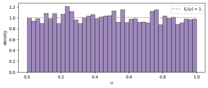
The histogram will not be perfectly flat because it is built from a finite sample. Still, it should hover around the theoretical density \(f_U(u)=1\). This is our first example of comparing an empirical distribution to the distribution we intended to sample.

Expectation and basic rules

Although detailed computation of expectations belongs to later lessons, we close by stating the definition of the expected value of a random variable \(X\). For discrete variables

\[E[X] = \sum_{x} x\,f_X(x)\,,\]

and for continuous variables

\[E[X] = \int_{-\infty}^{\infty} x\,f_X(x)\,dx\,.\]

Expectation is a linear operator: \(E[aX + bY] = aE[X] + bE[Y]\). We will make use of these rules when we build sampling and estimator formulas in later lessons.

For now, expectation should be read as the model’s long-run average value. It is not necessarily a value the random variable can actually take. A fair coin encoded as 0 for tails and 1 for heads has expected value \(0.5\), even though neither flip can produce the value 0.5.

Later we will also need quantities that measure spread around the expected value. The most important one is the variance,

\[\operatorname{Var}(X)=E[(X-E[X])^2]\,,\]

but we will wait until Lesson 08 to use it carefully for Monte Carlo uncertainty.

Looking ahead

In Lesson 07 we will learn how to sample from distributions other than \(U(0,1)\). Inverse-transform sampling uses the CDF to transform a uniform sample into an exponential flight distance or other random variable. We will also introduce histograms as empirical distributions and explore how bin count and sample size affect the appearance of a distribution. These tools will then feed back into our neutron simulation.

Before the next lesson, review the basic language of CDFs, PMFs, PDFs, support, and normalization. In Lesson 07 we will use the CDF more actively: instead of only describing a distribution, we will use it to generate samples from that distribution. The main target will be exponential flight distances, which are the next step toward a more physical neutron transport model.