Advection, Diffusion, and Reaction Models
Overview, Objectives, and Key Terms
Lesson 10 started with balance rows: what is in a cell comes from what enters, what leaves, what is created, and what is destroyed. Today we take the same bookkeeping seriously enough that it becomes a differential equation.
The central move is to count an amount in a small cell first, then decide how that amount changes. Once the units are right, the advection-diffusion-reaction equation is much less mysterious.
By the end of this lesson, you should be able to:
distinguish a density \(u(x,t)\) from a cell amount \(U_i(t)\),
write a one-dimensional integral balance over a fixed or moving cell,
identify advection, diffusion, and reaction terms by their units,
derive the fixed-coordinate ADR form from a flux balance,
recognize finite differences as one way to enforce the same local balance,
identify several reduced models as children of the same parent balance.
Key terms. control volume, density, cell amount, flux, advection, diffusion, reaction, source, finite volume, finite difference, upwind.
[ ]:
import numpy as np
import matplotlib.pyplot as plt
from matplotlib.patches import Rectangle, FancyArrowPatch, Circle
from pathlib import Path

COLORS = {
    "ink": "#1f2937",
    "muted": "#64748b",
    "grid": "#cbd5e1",
    "panel": "#f8fafc",
    "purple": "#512888",
    "orange": "#D55E00",
    "blue": "#2563eb",
    "green": "#059669",
    "red": "#dc2626",
    "gold": "#f2b84b",
}

def style_axes(ax):
    ax.spines["top"].set_visible(False)
    ax.spines["right"].set_visible(False)
    ax.spines["left"].set_color(COLORS["muted"])
    ax.spines["bottom"].set_color(COLORS["muted"])
    ax.tick_params(colors=COLORS["muted"])
    ax.xaxis.label.set_color(COLORS["ink"])
    ax.yaxis.label.set_color(COLORS["ink"])
    ax.title.set_color(COLORS["ink"])
The L10 Picture Still Works
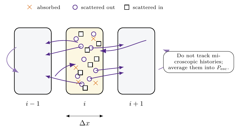
In L10, each row of a linear system was a balance over a cell. That diagram was not only a linear algebra story. It was also the seed of a partial differential equation story.
The only new idea is that the cell amount may now change with time and the cell faces may be allowed to move.
[ ]:
from IPython.display import Image, display

# L10 visual callback: microscopic motion averaged into cell-to-cell balance.
fig_path = Path("memos/figures/s10_escape_probability_sketch.png")
if not fig_path.exists():
    fig_path = Path("../../memos/figures/s10_escape_probability_sketch.png")

print("Input")
print(f"L10 figure path exists: {fig_path.exists()}")
print("Output")
print("Microscopic motion is being averaged into a face-to-face balance.")
if fig_path.exists():
    display(Image(filename=str(fig_path), width=720))
Input
L10 figure path exists: True
Output
Microscopic motion is being averaged into a face-to-face balance.
Count Beans Before Writing Derivatives
Let \(u(x,t)\) be a one-dimensional density. If we are tracking beans along a pipe, a useful unit is
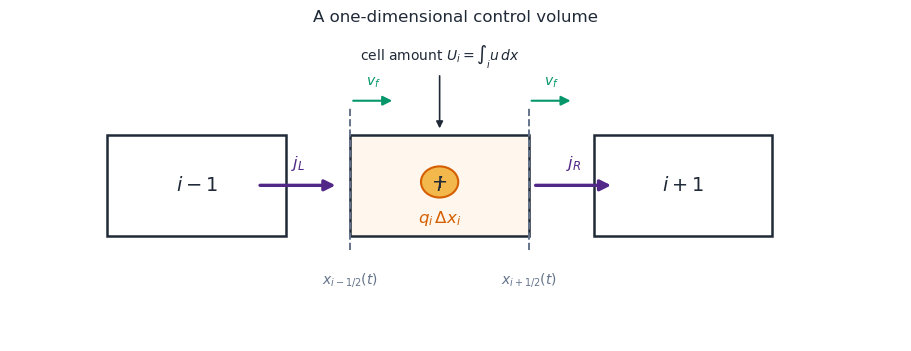
For a cell with left and right faces \(x_L(t)\) and \(x_R(t)\), the amount in the cell is
The units are now beans. That distinction is not cosmetic:
Every term in the balance must have those same units.
[ ]:
def draw_control_volume(ax):
    ax.set_xlim(-0.5, 10.5)
    ax.set_ylim(-1.3, 3.3)
    ax.axis("off")

    # neighbors and active cell
    for x, label, fill in [(0.7, "$i-1$", "#ffffff"), (3.7, "$i$", "#fff7ed"), (6.7, "$i+1$", "#ffffff")]:
        rect = Rectangle((x, 0.25), 2.2, 1.5, facecolor=fill, edgecolor=COLORS["ink"], lw=1.8)
        ax.add_patch(rect)
        ax.text(x+1.1, 1.0, label, ha="center", va="center", fontsize=14, color=COLORS["ink"])

    # moving faces
    for x, label in [(3.7, "$x_{i-1/2}(t)$"), (5.9, "$x_{i+1/2}(t)$")]:
        ax.plot([x, x], [0.05, 2.15], ls="--", color=COLORS["muted"], lw=1.4)
        ax.text(x, -0.25, label, ha="center", va="top", fontsize=10, color=COLORS["muted"])
        ax.add_patch(FancyArrowPatch((x, 2.25), (x+0.55, 2.25), arrowstyle="-|>", mutation_scale=14, lw=1.5, color=COLORS["green"]))
        ax.text(x+0.28, 2.48, "$v_f$", ha="center", fontsize=10, color=COLORS["green"])

    # flux arrows
    ax.add_patch(FancyArrowPatch((2.55, 1.0), (3.55, 1.0), arrowstyle="-|>", mutation_scale=16, lw=2.4, color=COLORS["purple"]))
    ax.add_patch(FancyArrowPatch((5.95, 1.0), (6.95, 1.0), arrowstyle="-|>", mutation_scale=16, lw=2.4, color=COLORS["purple"]))
    ax.text(3.05, 1.27, "$j_L$", ha="center", color=COLORS["purple"], fontsize=12)
    ax.text(6.45, 1.27, "$j_R$", ha="center", color=COLORS["purple"], fontsize=12)

    # source and reaction inside
    circ = Circle((4.8, 1.05), 0.23, facecolor=COLORS["gold"], edgecolor=COLORS["orange"], lw=1.5)
    ax.add_patch(circ)
    ax.text(4.8, 1.05, "+", ha="center", va="center", fontsize=14, color=COLORS["ink"])
    ax.text(4.8, 0.45, "$q_i\\,\\Delta x_i$", ha="center", fontsize=12, color=COLORS["orange"])

    ax.annotate("cell amount $U_i=\\int_i u\\,dx$", xy=(4.8, 1.8), xytext=(4.8, 2.85),
                ha="center", color=COLORS["ink"],
                arrowprops=dict(arrowstyle="-|>", lw=1.2, color=COLORS["ink"]))
    ax.set_title("A one-dimensional control volume", color=COLORS["ink"])

fig, ax = plt.subplots(figsize=(9, 3.4), constrained_layout=True)
draw_control_volume(ax)
plt.show()
The Integral Balance
Use \(j(x,t)\) for the rightward physical flow through a face. In one dimension, its units are
If a face itself moves with speed \(v_f=dx_f/dt\), then material swept along by the moving face contributes \(u v_f\). The relative flow across that face is
The one-dimensional moving-cell balance is
Read it in words:
If the cell is fixed in space, \(v_f=0\), and this collapses to the more familiar fixed-control-volume balance.
Mechanisms Are Easier When Units Lead
A common closure for the face flow is
The two pieces mean different things:
\(w u\) is advection: material is carried by a velocity \(w\).
\(-D u_x\) is diffusion: material spreads down a gradient.
A simple net local source is
Here \(s\) creates material and \(\sigma u\) removes it. In a neutron setting we might call the removal an absorption or reaction rate. In a general ADR model, “reaction” just means local creation or destruction.
[ ]:
# Input: representative units in a one-dimensional unit-area model.
units = {
    "u": "beans / cm",
    "U_i = integral u dx": "beans",
    "w": "cm / s",
    "D": "cm^2 / s",
    "j = w u - D u_x": "beans / s",
    "s": "beans / (cm s)",
    "sigma": "1 / s",
    "sigma u": "beans / (cm s)",
}

print("Input")
print("Check each model term before trusting the equation.")
print("Output")
for name, unit in units.items():
    print(f"{name:24s}: {unit}")
Input
Check each model term before trusting the equation.
Output
u                       : beans / cm
U_i = integral u dx     : beans
w                       : cm / s
D                       : cm^2 / s
j = w u - D u_x         : beans / s
s                       : beans / (cm s)
sigma                   : 1 / s
sigma u                 : beans / (cm s)
From Integral Balance to Continuum Model
For a fixed cell, the integral balance is
Shrinking the cell gives the differential balance
Now substitute the closure choices:
The general one-dimensional ADR model is
If \(w\), \(D\), and \(\sigma\) are constant, this becomes
The equation looks compact, but it is still bean counting.
One Parent Balance, Several Child Models
The parent equation is useful because we can simplify it in controlled ways. A “cell” does not always have to be a spatial volume. It can also be an isotope name, a precursor group, an energy bin, or any state that owns an amount.
The linear pattern is the same as long as rates are proportional to the current unknowns and the source terms are known.
Assumptions |
Reduced balance |
Mathematical type |
Physical reading |
|---|---|---|---|
steady, no spatial variation |
\(\Sigma u=s_0\) |
algebraic balance |
infinite-medium production equals removal |
time-dependent, no spatial variation |
\(u'=-\Sigma u+s_0\) |
first-order IVP |
well-mixed point model |
steady 1-D, no diffusion |
\(w u' + \Sigma u=s_0\) |
first-order ODE with inflow data |
advection-reaction in a flow |
steady 1-D, no advection |
\(-D u''+\Sigma u=s_0\) |
second-order BVP |
reaction-diffusion in a slab |
time-dependent, named states |
\(\mathbf{y}'=A\mathbf{y}+\mathbf{q}\) |
linear system of IVPs |
isotope chains / precursor groups |
The point is not to memorize a menu. The point is to see the family resemblance: every line is still a balance.
[ ]:
# Input: a small menu of linear balances descended from the same ADR parent.
models = [
    ("infinite-medium reaction", "Sigma*u = s0", "algebraic"),
    ("well-mixed inventory", "u' = -Sigma*u + s0", "IVP"),
    ("1-D flow", "w*u' + Sigma*u = s0", "first-order ODE"),
    ("1-D slab diffusion", "-D*u'' + Sigma*u = s0", "BVP"),
    ("named isotope chain", "y' = A@y + q", "linear IVP system"),
]

print("Input")
print("Start from accumulation = inflow - outflow + creation - removal.")
print("Output")
for name, equation, kind in models:
    print(f"{name:26s} -> {equation:28s} ({kind})")
Input
Start from accumulation = inflow - outflow + creation - removal.
Output
infinite-medium reaction   -> Sigma*u = s0                 (algebraic)
well-mixed inventory       -> u' = -Sigma*u + s0           (IVP)
1-D flow                   -> w*u' + Sigma*u = s0          (first-order ODE)
1-D slab diffusion         -> -D*u'' + Sigma*u = s0        (BVP)
named isotope chain        -> y' = A@y + q                 (linear IVP system)
Named-State Balances: U-238 to Pu-239 as a Linear Chain
A spatial cell is not the only kind of bookkeeping box. We can also balance named populations. A simplified transmutation chain might fold short-lived details into three buckets:
This is not a depletion-grade reactor model. It is a clean linear balance example. Let
If \(\gamma_U\) converts U-238 into the next bucket, \(\lambda_{Np}\) converts Np-239 into Pu-239, and \(\rho_{Pu}\) removes Pu-239, then
The rows are still balances. The off-diagonal entries are transfers between names instead of transfers between neighboring volumes.
[ ]:
# Input: simplified named-state chain rates.
gamma_u = 0.020      # 1/day, effective conversion out of U-238 bucket
lambda_np = 0.35     # 1/day, Np-239 to Pu-239 bucket
rho_pu = 0.004       # 1/day, effective Pu-239 removal
N = np.array([100.0, 2.0, 0.5])
q = np.array([0.0, 0.0, 0.0])

A_chain = np.array([
    [-gamma_u, 0.0, 0.0],
    [ gamma_u, -lambda_np, 0.0],
    [ 0.0, lambda_np, -rho_pu],
])
dNdt = A_chain @ N + q

print("Input")
print(f"state [U-238, Np-239, Pu-239] = {N}")
print("Output")
print("A =")
print(A_chain)
print(f"dN/dt = {np.round(dNdt, 4)} per day")
print(f"total named inventory rate = {np.sum(dNdt):.4f} per day")
Input
state [U-238, Np-239, Pu-239] = [100.    2.    0.5]
Output
A =
[[-0.02   0.     0.   ]
 [ 0.02  -0.35   0.   ]
 [ 0.     0.35  -0.004]]
dN/dt = [-2.     1.3    0.698] per day
total named inventory rate = -0.0020 per day
Geometry Changes the Weights, Not the Bookkeeping
The same PDE idea also generalizes by changing the geometry. In one-dimensional slab geometry, fixed cells have equal volume per unit area, so the balance uses widths like \(\Delta x\).
For radial diffusion in a cylinder, the shell volume and face area depend on radius. With radial symmetry and no advection,
The term looks different, but the story is the same: accumulation in a thin annular shell is driven by what crosses the inner face, what crosses the outer face, and what is created or removed inside. Geometry changes the face areas and volumes. It does not change the balance habit.
Finite Differences Enforce the Same Balance
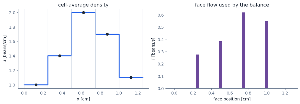
On a uniform fixed grid with width \(\Delta x\), let \(u_i\) approximate the cell-average density. Then
The finite-volume balance is
A finite-difference method supplies approximations for the face flows. For diffusion,
For positive advection speed \(w>0\), the upwind face flow is
That is still a balance statement. We have only chosen how to estimate the two face terms.
[ ]:
# Input: a five-cell profile and simple ADR data.
dx = 0.25                 # cm
w = 0.30                  # cm/s, positive means motion to the right
D = 0.015                 # cm^2/s
sigma = 0.08              # 1/s
u = np.array([1.0, 1.4, 2.0, 1.7, 1.1])  # beans/cm
s = np.array([0.0, 0.15, 0.25, 0.10, 0.0]) # beans/(cm s)

# Upwind advection and centered diffusion at interior faces.
# Boundary face flows are set to zero here so the example stays compact.
F = np.zeros(len(u)+1)
for face in range(1, len(u)):
    u_left = u[face-1]
    u_right = u[face]
    F_adv = w * u_left
    F_diff = -D * (u_right - u_left) / dx
    F[face] = F_adv + F_diff

du_dt = (F[:-1] - F[1:]) / dx + s - sigma*u

print("Input")
print(f"dx={dx:.2f} cm, w={w:.2f} cm/s, D={D:.3f} cm^2/s, sigma={sigma:.2f} 1/s")
print(f"u={u}")
print("Output")
print(f"face flows F={np.round(F, 4)} beans/s")
print(f"du/dt={np.round(du_dt, 4)} beans/(cm s)")
print(f"net amount rate={np.sum(du_dt)*dx:.4f} beans/s")

x_centers = (np.arange(len(u)) + 0.5)*dx
x_faces = np.arange(len(u)+1)*dx
fig, axes = plt.subplots(1, 2, figsize=(10, 3.4), constrained_layout=True)
ax = axes[0]
ax.step(np.r_[0, x_centers, len(u)*dx], np.r_[u[0], u, u[-1]], where="mid", color=COLORS["blue"], lw=2.4)
ax.scatter(x_centers, u, color=COLORS["ink"], zorder=3)
for xf in x_faces:
    ax.axvline(xf, color=COLORS["grid"], lw=1)
ax.set_xlabel("x [cm]")
ax.set_ylabel("u [beans/cm]")
ax.set_title("cell-average density")
style_axes(ax)

ax = axes[1]
ax.axhline(0, color=COLORS["ink"], lw=1)
ax.bar(x_faces, F, width=0.035, color=COLORS["purple"], alpha=0.85)
ax.set_xlabel("face position [cm]")
ax.set_ylabel("F [beans/s]")
ax.set_title("face flow used by the balance")
style_axes(ax)
plt.show()
Input
dx=0.25 cm, w=0.30 cm/s, D=0.015 cm^2/s, sigma=0.08 1/s
u=[1.  1.4 2.  1.7 1.1]
Output
face flows F=[0.    0.276 0.384 0.618 0.546 0.   ] beans/s
du/dt=[-1.184 -0.394 -0.846  0.252  2.096] beans/(cm s)
net amount rate=-0.0190 beans/s
A Steady Diffusion-Reaction Row
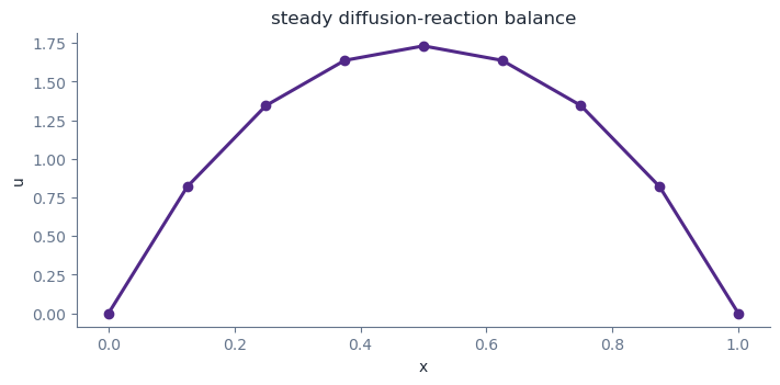
If advection is absent and the model is steady, the fixed-coordinate ADR equation reduces to
The centered finite-difference row at an interior point is
That row should feel familiar from L10. It is the same nearest-neighbor balance pattern: left neighbor, center cell, right neighbor, and a known source.
[ ]:
# Input: solve a small steady diffusion-reaction boundary-value problem.
length = 1.0
num_interior = 7
D = 0.04
sigma = 0.30
source_strength = 1.0
left_value = 0.0
right_value = 0.0

dx = length/(num_interior + 1)
x = np.linspace(dx, length-dx, num_interior)
main = (2*D/dx**2 + sigma) * np.ones(num_interior)
off = (-D/dx**2) * np.ones(num_interior-1)
A = np.diag(main) + np.diag(off, 1) + np.diag(off, -1)
b = source_strength * np.ones(num_interior)
b[0] += D/dx**2 * left_value
b[-1] += D/dx**2 * right_value
u_interior = np.linalg.solve(A, b)
residual = A @ u_interior - b

x_plot = np.r_[0.0, x, length]
u_plot = np.r_[left_value, u_interior, right_value]

print("Input")
print(f"N={num_interior}, dx={dx:.3f}, D={D:.3f}, sigma={sigma:.3f}, source={source_strength:.3f}")
print("Output")
print(f"max residual magnitude = {np.max(np.abs(residual)):.2e}")
print(f"center value = {u_interior[len(u_interior)//2]:.4f}")

fig, ax = plt.subplots(figsize=(7, 3.4), constrained_layout=True)
ax.plot(x_plot, u_plot, color=COLORS["purple"], marker="o", lw=2.2)
ax.set_xlabel("x")
ax.set_ylabel("u")
ax.set_title("steady diffusion-reaction balance")
style_axes(ax)
plt.show()
Input
N=7, dx=0.125, D=0.040, sigma=0.300, source=1.000
Output
max residual magnitude = 1.11e-15
center value = 1.7318
What To Carry Forward
ADR is a balance law with three mechanisms: carry, spread, create/destroy.
Units decide whether a term belongs in the equation.
The integral balance is often the safest starting point because it counts an amount in a cell.
The differential equation appears when we shrink the fixed cell.
Finite differences and finite volumes are not just formulas for derivatives. They are numerical ways to enforce the same balance on a grid.
Next, we will use this kind of model as a reason to solve differential equations, first symbolically and then numerically.