Lesson 12 - One Matrix, Many Scenarios
Learning goals. By the end of this lecture, students should be able to:
explain why one coefficient matrix may be reused with many right-hand sides,
describe Gaussian elimination as a process that decouples a linear system,
solve triangular systems by forward and back substitution,
interpret \(\mathbf{A}=\mathbf{L}\mathbf{U}\) as stored elimination work,
use residuals to check solutions for one or many right-hand sides.
Key terms. multiple right-hand sides, Gaussian elimination, triangular solve, LU factorization, pivoting.
The repeated-solve pattern
In Lesson 10, one model produced one linear system,
In practice, the matrix \(\mathbf{A}\) often stays fixed while the right-hand side changes. A source moves. A boundary value changes. A forcing term is adjusted. A sensitivity calculation asks how the response changes under several scenarios. In an engineering design study, this means the geometry, materials, and coupling model may stay fixed while the operating case changes.
The resulting problems have the form
If the expensive work depends only on \(\mathbf{A}\), we should do that work once and reuse it.
A small example with several sources
Return to the four-cell balance matrix from Lesson 10, with \(c=0.8\):
Now compare three source scenarios:
The first source enters from the left. The second source enters from the right. The third source is distributed uniformly through the four cells. Here the three right-hand sides use the same source-normalized units; \(\mathbf{b}_3\) spreads one total source unit evenly over four cells. The physics of transport between cells is unchanged, so \(\mathbf{A}\) is unchanged.
If we collect the right-hand sides into a matrix,
then solving
solves all three scenarios at once. Column \(j\) of \(\mathbf{B}\) is one source scenario, and column \(j\) of \(\mathbf{X}\) is the corresponding state or response field.
This is the same source-response idea introduced in Lesson 10. If \(\mathbf{M}=\mathbf{A}^{-1}\), then \(\mathbf{X}=\mathbf{M}\mathbf{B}\): each solution column is a linear combination of unit-source response columns. That is the conceptual interpretation, not the recommended computational route. The practical question in this lecture is how to reuse matrix-dependent work without explicitly forming \(\mathbf{M}\).
[1]:
import numpy as np

c = 0.8
A = np.array([[1.0, -c/2, 0.0, 0.0],
              [-c/2, 1.0, -c/2, 0.0],
              [0.0, -c/2, 1.0, -c/2],
              [0.0, 0.0, -c/2, 1.0]])
b1 = np.array([1.0, 0.0, 0.0, 0.0])
b2 = np.array([0.0, 0.0, 0.0, 1.0])
b3 = np.array([0.25, 0.25, 0.25, 0.25])
B = np.column_stack((b1, b2, b3))

X = np.linalg.solve(A, B)
R = B - A @ X
print(X)
print(np.linalg.norm(R))
[[1.24633431 0.11730205 0.56818182]
 [0.61583578 0.29325513 0.79545455]
 [0.29325513 0.61583578 0.79545455]
 [0.11730205 1.24633431 0.56818182]]
1.3611050621282487e-16
Worked example: interpreting the solution columns
Problem. For the three right-hand sides above, solve \(\mathbf{A}\mathbf{X}=\mathbf{B}\), identify which source each column represents, and check the balances with a residual.
Solution. The computed solution matrix is approximately
The first column is the response to the left source, and the second column is the mirror-image response to the right source. The third column is larger in the middle because the source is distributed through the whole domain while leakage still occurs at the ends.
The residual matrix
checks all three scenarios at once. For example, the first column checks the balance equations for the left-source case. Each residual column has the same units as the corresponding source column in \(\mathbf{B}\). Numerically, the Frobenius norm \(\lVert\mathbf{R}\rVert_F\) is about \(10^{-16}\), so the displayed solutions satisfy the balances to roundoff.
Elimination: removing coupling step by step
Gaussian elimination transforms a coupled system into an equivalent triangular system. For example, consider
The row operations below are algebraic bookkeeping. After elimination, the triangular rows no longer need to look like the original physical cell balances, so residual checks should use the original \(\mathbf{A}\).
The first equation is \(2x_1-x_2=1\). The second equation contains \(x_1\). To remove it, add one half of the first row to the second row:
As a matrix operation on the augmented system,
Next, use the new second row to remove \(x_2\) from the third row. The multiplier is \(-1/(3/2)=-2/3\), so add \(2/3\) of row 2 to row 3:
The resulting upper-triangular system is
This upper-triangular system is much easier to solve.
Augmented matrices for bookkeeping
When doing elimination by hand, it is easy to lose track of the right-hand side. An augmented matrix keeps the coefficients and right-hand side together:
Row operations are applied to the whole row, including the right-hand side column. After the two elimination steps above, the augmented matrix becomes
The left block is the upper-triangular matrix \(\mathbf{U}\), and the right column is the transformed right-hand side.
If we also want to record the elimination multipliers, we can store them in the lower-left entries that were just eliminated:
The upper triangle stores \(\mathbf{U}\). The lower entries \(-1/2\) and \(-2/3\) store the LU multipliers from the original rows. In the row-operation notation above we added \(+1/2\) of row 1 and \(+2/3\) of row 2 to cancel those entries; the stored LU multipliers have the opposite sign because they record the original subdiagonal coefficient divided by the pivot. Once stored, they are fixed data, not entries to eliminate again. This is the storage idea behind LU factorization. The augmented matrix is a useful scratchpad; the factors \(\mathbf{L}\) and \(\mathbf{U}\) are the reusable result.
Back substitution
A triangular system can be solved from the bottom up. From the last row,
so \(x_3=1\). The second row gives
so \(x_2=1\). The first row gives
so \(x_1=1\). Thus
The same calculation can be written as an algorithm.
Algorithm: Back substitution for \(\mathbf{U}\mathbf{x}=\mathbf{y}\)
Start with the last row.
Solve for the last unknown.
Move upward one row at a time.
In each row, subtract the contributions from already-known unknowns.
Divide by the diagonal entry.
From elimination to LU
Elimination produces an upper-triangular matrix \(\mathbf{U}\). The multipliers used during elimination can be stored in a lower-triangular matrix \(\mathbf{L}\). Together, they give a factorization
For the previous example,
The signs in \(\mathbf{L}\) record the LU multipliers from the original rows. The row-operation matrices used above satisfy \(\mathbf{E}_{32}\mathbf{E}_{21}\mathbf{A}=\mathbf{U}\), while the LU factor uses the inverse operations, \(\mathbf{L}=\mathbf{E}_{21}^{-1}\mathbf{E}_{32}^{-1}\). Different sign conventions are possible depending on how the elimination steps are written, but the idea is the same: \(\mathbf{L}\) and \(\mathbf{U}\) store the reusable work.
Once \(\mathbf{A}=\mathbf{L}\mathbf{U}\), solving \(\mathbf{A}\mathbf{x}=\mathbf{b}\) becomes two triangular solves:
The first is solved by forward substitution. The second is solved by back substitution.
Takeaway. LU factorization separates the solve into two parts: expensive work that depends on \(\mathbf{A}\), and cheaper triangular solves that can be repeated for each new right-hand side.
[2]:
A_small = np.array([[2.0, -1.0, 0.0],
                    [-1.0, 2.0, -1.0],
                    [0.0, -1.0, 2.0]])
L_small = np.array([[1.0, 0.0, 0.0],
                    [-0.5, 1.0, 0.0],
                    [0.0, -2.0/3.0, 1.0]])
U_small = np.array([[2.0, -1.0, 0.0],
                    [0.0, 1.5, -1.0],
                    [0.0, 0.0, 4.0/3.0]])

print(L_small @ U_small)
print(np.allclose(L_small @ U_small, A_small))
[[ 2. -1.  0.]
 [-1.  2. -1.]
 [ 0. -1.  2.]]
True
Pivoting
At each elimination step, the pivot is the diagonal entry used to eliminate entries below it. Elimination divides by pivot entries. If a pivot is zero, the naive algorithm breaks down. If a pivot is very small, the algorithm may be numerically unstable. Practical solvers therefore use pivoting: they swap rows to place a better pivot in the current position.
With pivoting, the factorization is often written
where \(\mathbf{P}\) is a permutation matrix that records row swaps. Students do not need to implement a production-quality pivoting strategy in this course, but they should recognize that pivoting is one reason library routines are preferred for practical work. Plainly: numerical solutions are sometimes more accurate if the equations are reordered before elimination.
Using SciPy for reusable solves
SciPy exposes the factor-and-reuse pattern directly.
[3]:
from scipy.linalg import lu_factor, lu_solve

A_lu = np.array([[2.0, -1.0, 0.0],
                 [-1.0, 2.0, -1.0],
                 [0.0, -1.0, 2.0]])
B_lu = np.array([[1.0, 0.0],
                 [0.0, 0.0],
                 [1.0, 1.0]])

lu, piv = lu_factor(A_lu)
X_lu = lu_solve((lu, piv), B_lu)
R_lu = B_lu - A_lu @ X_lu
print(X_lu)
print(np.linalg.norm(R_lu))
[[1.   0.25]
 [1.   0.5 ]
 [1.   0.75]]
2.9373740229761033e-16
The call to lu_factor performs the matrix-dependent work. The call to lu_solve applies the factorization to the right-hand side. If another right-hand side vector or matrix is needed later, the same factors can be reused.
Why not compute the inverse?
It is tempting to write
This is mathematically correct when \(\mathbf{A}\) is invertible, but it is usually not the best computational instruction. Forming \(\mathbf{A}^{-1}\) explicitly is more expensive, can be less stable, and often destroys sparsity. For sparse transport or diffusion matrices, the inverse generally becomes dense, obscuring locality and wasting memory. In practical numerical linear algebra, we solve systems; we do not form inverses unless there is a special reason.
The cost difference is important. Factoring a dense \(n\times n\) matrix costs on the order of \(n^3\) operations. Once the factorization is available, one triangular solve with a single right-hand side costs on the order of \(n^2\). For \(k\) right-hand sides, factor-and-reuse work therefore has the form \(O(n^3+k n^2)\). Forming an explicit inverse effectively solves against all \(n\) unit-source right-hand sides, stores those dense response columns, and then multiplies by the particular \(\mathbf{b}\).
[4]:
import numpy as np

n = 300
rng = np.random.default_rng(2)
A_timing = rng.random((n, n)) + n*np.eye(n)
b_timing = rng.random(n)

# In Jupyter/IPython:
# %timeit np.linalg.solve(A_timing, b_timing)
# %timeit np.linalg.inv(A_timing) @ b_timing
This benchmark compares a fresh direct solve with forming an explicit inverse for one right-hand side. It does not show the separate factor-and-reuse advantage of lu_factor and lu_solve, because np.linalg.solve(A, b) refactors \(\mathbf{A}\) each timing run.
\(n\) |
direct solve |
inverse route |
inverse/direct |
|---|---|---|---|
100 |
\(0.033\ \mathrm{ms}\) |
\(0.100\ \mathrm{ms}\) |
\(3.0\times\) |
300 |
\(0.425\ \mathrm{ms}\) |
\(1.609\ \mathrm{ms}\) |
\(3.8\times\) |
1000 |
\(12.3\ \mathrm{ms}\) |
\(46.1\ \mathrm{ms}\) |
\(3.7\times\) |
3000 |
\(316\ \mathrm{ms}\) |
\(1171\ \mathrm{ms}\) |
\(3.7\times\) |
10000 |
\(10.5\ \mathrm{s}\) |
\(40.3\ \mathrm{s}\) |
\(3.8\times\) |
These are representative dense solve timings from one WSL2 machine using Python 3.13, NumPy 2.4, OpenBLAS, and one BLAS thread. Exact timings depend on hardware, BLAS library, cache behavior, problem size, and thread count; the \(n=10000\) inverse run also used several GB of memory.
The following cell reproduces the same comparison as a notebook-generated plot. The curves are normalized by their \(n=100\) timings and compared with the cubic reference curve \((n/100)^3\).
[5]:
import matplotlib.pyplot as plt

n_values = np.array([100, 300, 1000, 3000, 10000], dtype=float)
solve_times = np.array([0.033e-3, 0.425e-3, 12.3e-3, 316e-3, 10.5])
inverse_times = np.array([0.100e-3, 1.609e-3, 46.1e-3, 1171e-3, 40.3])

solve_relative = solve_times / solve_times[0]
inverse_relative = inverse_times / inverse_times[0]
cubic_reference = (n_values / n_values[0])**3

fig, ax = plt.subplots(figsize=(6.5, 4.0))
ax.loglog(n_values, solve_relative, "o-", label="solve")
ax.loglog(n_values, inverse_relative, "s-", label="inverse route")
ax.loglog(n_values, cubic_reference, "--", label=r"$(n/100)^3$")
ax.set_xlabel("matrix size $n$")
ax.set_ylabel("time relative to $n=100$")
ax.grid(True, which="both", alpha=0.3)
ax.legend()
fig.tight_layout()
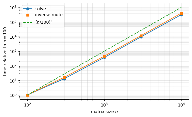
Another way to read the same data is to compare adjacent rows. A perfectly cubic time would grow by \((n_i/n_{i-1})^3\):
step |
\((n_i/n_{i-1})^3\) |
solve growth |
inverse-route growth |
|---|---|---|---|
\(100\rightarrow 300\) |
27.0 |
12.8 |
16.1 |
\(300\rightarrow 1000\) |
37.0 |
28.9 |
28.7 |
\(1000\rightarrow 3000\) |
27.0 |
25.7 |
25.4 |
\(3000\rightarrow 10000\) |
37.0 |
33.2 |
34.4 |
Both routes produce a mathematically related answer for this nonsingular matrix, but the inverse route does extra cubic-order work, stores a dense matrix, and can be less stable. In sparse transport and diffusion problems, the storage issue is often the decisive one.
The distinction is useful:
\(\mathbf{A}\) is the balance or operator matrix.
\(\mathbf{A}^{-1}\) is the conceptual response map from sources to solutions; if \(\mathbf{b}\) carries source units, it is a source-to-state response per unit source. Its entries are response coefficients, not probabilities; in source-normalized population models they may exceed one because they count expected visits or population per unit source.
LU factors are the practical stored work used to apply that response to one right-hand side after another.
This point returns in Lesson 14, where sparse matrices make the cost of explicit inverses especially visible.
Checking many solutions at once
When \(\mathbf{A}\mathbf{X}=\mathbf{B}\), the residual is a matrix:
Each column of \(\mathbf{R}\) is the residual for one right-hand side: a defect in the balance equations for one scenario. A matrix norm or column-by-column vector norms can be used to check the solve.
For example, if \(\mathbf{B}\) contains several source scenarios, then the residual columns audit the balance equations for each scenario. This is the same physical idea as before, just organized for several cases at once.
Exercises
Forward eliminate the entries below the diagonal in
\[\begin{split}\mathbf{A}_1=\begin{bmatrix} 2&1&0\\ 4&5&1\\ 0&2&3 \end{bmatrix}.\end{split}\]Forward eliminate the entries below the diagonal in
\[\begin{split}\mathbf{A}_2=\begin{bmatrix} 1&2&1\\ 3&8&2\\ 0&4&5 \end{bmatrix}.\end{split}\]Forward eliminate the entries below the diagonal in
\[\begin{split}\mathbf{A}_3=\begin{bmatrix} 1&0&1\\ 2&1&3\\ 1&1&2 \end{bmatrix}.\end{split}\]What happens to the final pivot?
Let
\[\begin{split}\mathbf{A}=\begin{bmatrix} 2&-1\\ -1&2 \end{bmatrix}, \qquad \mathbf{B}=\begin{bmatrix} 1&0\\ 0&1 \end{bmatrix}.\end{split}\]Solve \(\mathbf{A}\mathbf{X}=\mathbf{B}\), compute \(\mathbf{R}=\mathbf{B}-\mathbf{A}\mathbf{X}\), and state what each residual column checks.
Answers.
\(\mathbf{U}_1=\begin{bmatrix}2&1&0\\0&3&1\\0&0&7/3\end{bmatrix}\).
\(\mathbf{U}_2=\begin{bmatrix}1&2&1\\0&2&-1\\0&0&7\end{bmatrix}\).
\(\mathbf{U}_3=\begin{bmatrix}1&0&1\\0&1&1\\0&0&0\end{bmatrix}\). The final pivot is zero, so ordinary back substitution cannot determine a unique third unknown.
\(\mathbf{X}=\mathbf{A}^{-1}\mathbf{B}=\frac{1}{3}\begin{bmatrix}2&1\\1&2\end{bmatrix}\), so \(\mathbf{R}=\mathbf{0}\). The first residual column checks the balance equations for the first right-hand side, and the second residual column checks the second right-hand side.
End-of-lecture summary
Takeaway.
Many engineering studies reuse the same matrix with different right-hand sides.
Gaussian elimination removes coupling below the diagonal and produces an upper-triangular system.
Triangular systems are solved by forward or back substitution.
LU factorization stores elimination work so that new right-hand sides can be solved efficiently.
\(\mathbf{A}\) is the balance/operator matrix, \(\mathbf{A}^{-1}\) is the conceptual response map, and LU factors are the practical stored computational work.
Practical solvers use pivoting and should be checked with residuals.
Lesson 13 uses symbolic tools to inspect small systems and parameter dependence before returning to larger numerical methods.