Constrained Optimization
Overview, Objectives, and Key Terms
In Lesson 22, the question was simply, “Where is the objective function best?” That is already useful, but it is rarely the engineering question. Engineering problems usually sound more like this:
Find the best design we are allowed to use.
A constraint is an engineering promise: do not exceed this dose, do not ask for a negative thickness, do not violate a balance law, do not use more material than the system can hold.
Objectives
By the end of this lesson, you should be able to
identify design variables, objective functions, bounds, equality constraints, and inequality constraints,
translate technical specifications into the constraint convention used by
scipy.optimize.minimize,use
minimizefor small constrained optimization problems written as Python functions,recognize when a problem is a linear program and use
scipy.optimize.linprog,check solver output for success, feasibility, active constraints, and units.
Key Terms
objective function
design variable
feasible region
bound
equality constraint
inequality constraint
active constraint
linear programming
scipy.optimize.minimizescipy.optimize.linprog
Start With the minimize Convention
We will use minimize as the default language for constrained optimization. A typical problem is
subject to inequality constraints
equality constraints
and bounds
In minimize, an old-style inequality constraint has type: "ineq", and the function must return a value that is nonnegative when the constraint is satisfied. Equality constraints use type: "eq", and the function should return zero when the equality is satisfied.
That means the first job is translation. If a dose specification says \(D(\mathbf{x}) \le D_{\max}\), the minimize constraint function can be
Now the satisfied condition is \(g(\mathbf{x}) \ge 0\).
Where linprog Deviates
linprog is not wrong; it just speaks a different dialect. It wants the linear-programming form
subject to matrix rows
plus bounds. So a technical requirement like
is passed to linprog as
Same engineering statement, different solver convention.
Picking the Right SciPy Tool
Use minimize when the objective or constraints are most naturally written as Python functions. That includes nonlinear functions, tabulated models wrapped in interpolation, simulation-based objective functions, and cases where the feasible region is curved.
Use linprog when the objective and constraint functions are linear functions of \(\mathbf{x}\), then linprog and the linear-programming form are probably clearer.
The solver handles bookkeeping. We still own the variables, objective, and constraints.
[1]:
import numpy as np
import matplotlib.pyplot as plt
from scipy.optimize import Bounds, linprog, minimize

COLORS = {
    "ink": "#1f2937",
    "muted": "#64748b",
    "grid": "#e5e7eb",
    "panel": "#fafaf7",
    "purple": "#512888",
    "orange": "#D55E00",
    "blue": "#2563eb",
    "green": "#059669",
    "red": "#dc2626",
}

plt.rcParams.update({
    "figure.facecolor": "white",
    "figure.figsize": (8,3),
    "axes.facecolor": COLORS["panel"],
    "axes.edgecolor": COLORS["muted"],
    "axes.labelcolor": COLORS["ink"],
    "axes.titlecolor": COLORS["ink"],
    "xtick.color": COLORS["ink"],
    "ytick.color": COLORS["ink"],
    "grid.color": COLORS["grid"],
    "font.size": 11,
})


def style_axes(ax):
    ax.grid(True, alpha=0.55)
    ax.spines["top"].set_visible(False)
    ax.spines["right"].set_visible(False)
Case Study 1: When Should We Count an Activated Sample?
Technical Specification
A sample is removed from an irradiation position at \(t=0\). We must choose when to start a fixed-live-time count. The target signal decays moderately slowly. The interfering signal has a short-lived component, which clears quickly, and a smaller long-lived/background component, which does not disappear as fast.
Waiting can improve the target-to-interference balance at first, but waiting too long throws away the target. The detector also has a practical total-rate limit.
Let \(t\) be the delay, in hours, from sample removal to the start of counting. For this fixed live time, model the expected target and interfering counts as
[2]:
# Input block: signal model and limits for a one-time counting decision.
COUNTING_TIME_BOUNDS = (0.0, 72.0)   # h after removal from irradiation position
MIN_TARGET_COUNTS = 20.0             # relative counts
MAX_TOTAL_RATE = 85.0                # relative count-rate units
INITIAL_COUNTING_TIME = 18.0         # h


def target_counts(t):
    return 95.0*np.exp(-t/28.0)


def interfering_counts(t):
    return 220.0*np.exp(-t/7.0) + 18.0*np.exp(-t/85.0)


def total_rate(t):
    return target_counts(t) + interfering_counts(t)


def figure_of_merit(t):
    return target_counts(t) / np.sqrt(total_rate(t) + 1.0)


print("Input block")
print(f"time bounds        : {COUNTING_TIME_BOUNDS[0]:.0f} to {COUNTING_TIME_BOUNDS[1]:.0f} h")
print(f"minimum target     : {MIN_TARGET_COUNTS:.1f} relative counts")
print(f"maximum total rate : {MAX_TOTAL_RATE:.1f} relative count-rate units")
print(f"initial guess      : {INITIAL_COUNTING_TIME:.1f} h")
Input block
time bounds        : 0 to 72 h
minimum target     : 20.0 relative counts
maximum total rate : 85.0 relative count-rate units
initial guess      : 18.0 h
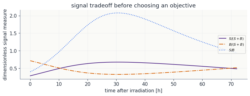
The plot below shows the tradeoff. The target fraction improves as the short-lived interference decays, but the target signal is also fading. These ratios help us see the physics; the optimization objective below uses a counting-statistics figure of merit.
[3]:
t_plt = np.linspace(COUNTING_TIME_BOUNDS[0], COUNTING_TIME_BOUNDS[1], 400)
c_target = target_counts(t_plt)
c_interfering = interfering_counts(t_plt)
c_total = total_rate(t_plt)

fig, ax = plt.subplots(figsize=(8, 3), constrained_layout=True)
ax.plot(t_plt, c_target/c_total, label="$S/(S+B)$", ls="-", color=COLORS["purple"])
ax.plot(t_plt, c_interfering/c_total, label="$B/(S+B)$", ls="-.", color=COLORS["orange"])
ax.plot(t_plt, c_target/c_interfering, label="$S/B$", ls=":", color=COLORS["blue"])
ax.set_xlabel("time after irradiation [h]")
ax.set_ylabel("dimensionless signal measure")
ax.set_title("signal tradeoff before choosing an objective")
ax.legend(fontsize=8, loc="center right")
style_axes(ax)
plt.show()
For this example, choose \(0 \le t \le 72\) hr to maximize
where \(S(t)\) is the target signal and \(B(t)\) is the interfering signal. The denominator is a simple Poisson-style uncertainty proxy for the total count, with a small regularizing term.
The constraints are:
target signal \(S(t) \ge 20\) relative counts,
total rate proxy \(S(t) + B(t) \le 85\) relative count-rate units.
Because the objective and constraints are Python functions of time, this is a minimize problem.
[4]:
# Model check block.
t_sample = np.array([0.0, 12.0, 24.0, 48.0], dtype=float)
target = target_counts(t_sample)
interference = interfering_counts(t_sample)
total = total_rate(t_sample)
fom = figure_of_merit(t_sample)

print("Model check")
for t, s, b, tot, f in zip(t_sample, target, interference, total, fom):
    print(f"t={t:4.0f} h: target={s:6.2f}, total={tot:6.2f}, FOM={f:5.2f}")
Model check
t=   0 h: target= 95.00, total=333.00, FOM= 5.20
t=  12 h: target= 61.89, total=117.14, FOM= 5.69
t=  24 h: target= 40.32, total= 61.02, FOM= 5.12
t=  48 h: target= 17.11, total= 27.57, FOM= 3.20
Translation to minimize
minimize passes the decision variables as a vector. Here \(x=[t]\), so the explicit inequality constraints are
The time limits \(0 \le x_0 \le 72\) are passed separately as bounds. The objective is also translated because minimize minimizes:
[5]:
def counting_objective(x):
    return -float(figure_of_merit(x[0]))

def enough_target_counts(x):
    # Technical spec: target_counts(t) >= MIN_TARGET_COUNTS
    # minimize ineq form: target_counts(t) - MIN_TARGET_COUNTS >= 0
    return float(target_counts(x[0]) - MIN_TARGET_COUNTS)


def not_too_much_total_rate(x):
    # Technical spec: total_rate(t) <= MAX_TOTAL_RATE
    # minimize ineq form: MAX_TOTAL_RATE - total_rate(t) >= 0
    return float(MAX_TOTAL_RATE - total_rate(x[0]))


counting_constraints = [
    {"type": "ineq", "fun": enough_target_counts},
    {"type": "ineq", "fun": not_too_much_total_rate},
]
counting_bounds = Bounds([COUNTING_TIME_BOUNDS[0]], [COUNTING_TIME_BOUNDS[1]])

print("Constraint translation at initial guess")
x0_counting = np.array([INITIAL_COUNTING_TIME])
print(f"objective(x0)              = {counting_objective(x0_counting): .4f}")
print(f"target-count margin g1(x0) = {enough_target_counts(x0_counting): .4f}")
print(f"rate-limit margin g2(x0)   = {not_too_much_total_rate(x0_counting): .4f}")
Constraint translation at initial guess
objective(x0)              = -5.5050
target-count margin g1(x0) =  29.9499
rate-limit margin g2(x0)   =  3.6716
[6]:
# Solve block.
counting_solution = minimize(
    counting_objective,
    x0=np.array([INITIAL_COUNTING_TIME]),
    bounds=counting_bounds,
    constraints=counting_constraints,
    method="SLSQP",
)

t_star = counting_solution.x[0]
[7]:
# Output/check block.
constraint_tol = 1e-8
target_margin = enough_target_counts([t_star])
rate_margin = not_too_much_total_rate([t_star])
lower_bound_margin = t_star - COUNTING_TIME_BOUNDS[0]
upper_bound_margin = COUNTING_TIME_BOUNDS[1] - t_star

print("Output block")
print(f"success: {counting_solution.success}")
print(f"message: {counting_solution.message}")
print(f"t* = {t_star:.3f} h")
print(f"minimized objective -FOM = {counting_solution.fun:.3f}")
print(f"figure of merit = {-counting_solution.fun:.3f}")
print(f"target counts = {target_counts(t_star):.2f}")
print(f"total rate proxy = {total_rate(t_star):.2f}")

for name, margin in [
    ("target-count g1", target_margin),
    ("rate-limit g2", rate_margin),
    ("lower time bound", lower_bound_margin),
    ("upper time bound", upper_bound_margin),
]:
    active = np.isclose(margin, 0.0, atol=constraint_tol)
    print(f"{name:18s}: margin={margin: .2e}, active={active}")
Output block
success: True
message: Optimization terminated successfully
t* = 17.189 h
minimized objective -FOM = -5.544
figure of merit = 5.544
target counts = 51.42
total rate proxy = 85.00
target-count g1   : margin= 3.14e+01, active=False
rate-limit g2     : margin=-2.84e-12, active=True
lower time bound  : margin= 1.72e+01, active=False
upper time bound  : margin= 5.48e+01, active=False
[8]:
t = np.linspace(COUNTING_TIME_BOUNDS[0], COUNTING_TIME_BOUNDS[1], 500)
feasible = (
    (target_counts(t) >= MIN_TARGET_COUNTS)
    & (total_rate(t) <= MAX_TOTAL_RATE)
)

fig, axes = plt.subplots(1, 2, figsize=(11, 3.8), constrained_layout=True)
ax = axes[0]
ax.plot(t, target_counts(t), color=COLORS["blue"], lw=2.5, label="target signal")
ax.plot(t, interfering_counts(t), color=COLORS["orange"], lw=2.5, label="interference/background")
ax.plot(t, total_rate(t), color=COLORS["muted"], lw=2, ls="--", label="total rate proxy")
ax.axhline(MAX_TOTAL_RATE, color=COLORS["red"], ls=":", lw=2, label="rate limit")
ax.axhline(MIN_TARGET_COUNTS, color=COLORS["green"], ls=":", lw=2, label="minimum target")
ax.axvline(t_star, color=COLORS["purple"], lw=2)
ax.set_xlabel("time after irradiation [h]")
ax.set_ylabel("relative counts")
ax.set_title("signals and constraints")
ax.legend(fontsize=8, loc="upper right")
style_axes(ax)

ax = axes[1]
ax.fill_between(t, 0, figure_of_merit(t), where=feasible, color=COLORS["green"], alpha=0.18, label="feasible window")
ax.fill_between(t, 0, figure_of_merit(t), where=~feasible, color=COLORS["red"], alpha=0.10, label="infeasible")
ax.plot(t, figure_of_merit(t), color=COLORS["purple"], lw=2.5, label="objective to maximize")
ax.plot(t_star, figure_of_merit(t_star), marker="*", ms=16, color=COLORS["green"], mec=COLORS["ink"], label="chosen time")
ax.set_xlabel("time after irradiation [h]")
ax.set_ylabel("signal separation proxy")
ax.set_title("best feasible counting time")
ax.legend(fontsize=8, loc="upper right")
style_axes(ax)
plt.show()
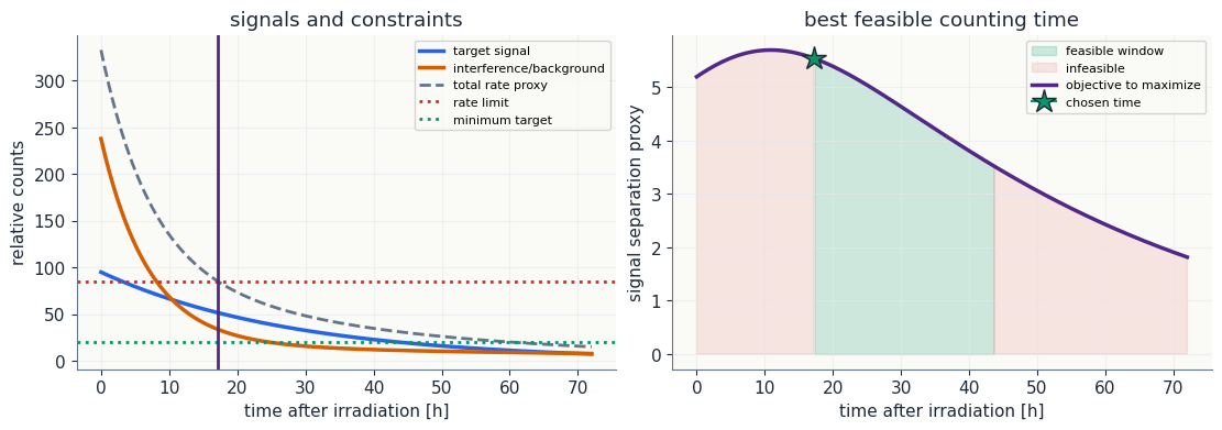
The rate-limit constraint is active: its margin is zero within numerical tolerance. The target-count constraint still has about 31 relative counts of slack, and neither time bound is active.
Physically, the detector-rate limit forces us to wait until the short-lived interference has dropped far enough. After that point, waiting longer mostly throws away target signal, so the figure of merit is already decreasing.
Boundaries, Active Constraints, and a Tiny Bit of Theory
For unconstrained optimization, we looked for places where the derivative or gradient vanished. With constraints, the optimum can sit on a boundary. In that case, the best feasible move may be no move at all, even if the unconstrained gradient is not zero.
That idea is the beginning of the Karush-Kuhn-Tucker conditions, usually abbreviated KKT. For this course, the important picture is enough:
an interior optimum behaves like the unconstrained case,
a boundary optimum is held in place by one or more active constraints,
for convex problems, a local optimum has much stronger global meaning,
for nonconvex problems, the initial guess and sanity checks matter more.
We do not need to turn KKT into another hand-calculation method. We need enough of it to read solver answers intelligently.
Example 2: Minimum-Cost Shielding With a Nonlinear Dose Response
Technical Specification
Now let \(\mathbf{x} = [x_w, x_s]^T\), where \(x_w\) is water thickness and \(x_s\) is steel thickness. The design goal is to minimize an installed cost index while keeping a dose-rate proxy below a design constraint.
The dose model is inspired by point-kernel shielding calculations:
where \(\tau = \mu_w x_w + \mu_s x_s\) is the optical thickness and \(B(\tau)\) is a simple buildup factor. Real shielding work uses energy-dependent attenuation coefficients and buildup-factor data; here we keep a one-energy teaching surrogate so the optimization structure is visible.
The technical constraints are:
shielded dose \(\le D_{\max}\),
total added thickness \(\le 35\) cm,
\(0 \le x_w \le 30\) cm,
\(0 \le x_s \le 8\) cm.
This is a minimize problem because the dose response includes thickness-dependent buildup.
[9]:
# Input block: technical specification for a simplified gamma-shielding problem.
# Variables are x = [water thickness, steel thickness], both in cm.
D0 = 100.0                       # mrem/h, unshielded dose-rate proxy
D_LIMIT = 2.0                    # mrem/h, design dose-rate constraint
MU = np.array([0.086, 0.58])     # cm^-1, rounded one-energy teaching values
BETA_BUILDUP = 0.25              # simple buildup-factor coefficient
MATERIAL_COST = np.array([1.0, 8.0])  # relative cost per cm for water and steel
BULK_PENALTY = 0.005             # installed bulk/space penalty
MAX_TOTAL_THICKNESS = 35.0       # cm
MAX_WATER_THICKNESS = 30.0       # cm
MAX_STEEL_THICKNESS = 8.0        # cm
INITIAL_SHIELD = np.array([20.0, 5.0])

print("Input block")
print(f"dose limit        : {D_LIMIT:.2f} mrem/h")
print(f"mu values         : water={MU[0]:.3f} cm^-1, steel={MU[1]:.3f} cm^-1")
print(f"cost coefficients : water={MATERIAL_COST[0]:.1f}, steel={MATERIAL_COST[1]:.1f}")
print(f"thickness limits  : total <= {MAX_TOTAL_THICKNESS:.1f} cm, steel <= {MAX_STEEL_THICKNESS:.1f} cm")
Input block
dose limit        : 2.00 mrem/h
mu values         : water=0.086 cm^-1, steel=0.580 cm^-1
cost coefficients : water=1.0, steel=8.0
thickness limits  : total <= 35.0 cm, steel <= 8.0 cm
[10]:
# Response model block: point-kernel-inspired attenuation with a simple buildup factor.
# This is a screening-level teaching model, not a shielding design standard.
def optical_thickness(x):
    x = np.asarray(x, dtype=float)
    return float(MU @ x)


def buildup_factor(x):
    tau = optical_thickness(x)
    return 1.0 + BETA_BUILDUP*tau


def shielded_dose(x):
    tau = optical_thickness(x)
    return D0*buildup_factor(x)*np.exp(-tau)


def shield_cost(x):
    x = np.asarray(x, dtype=float)
    return float(MATERIAL_COST @ x + BULK_PENALTY*np.sum(x)**2)


for x in [np.array([0.0, 0.0]), INITIAL_SHIELD, np.array([30.0, 3.5])]:
    print(f"x={x}: dose={shielded_dose(x):7.4f} mrem/h, cost={shield_cost(x):7.2f}, tau={optical_thickness(x):5.2f}")
x=[0. 0.]: dose=100.0000 mrem/h, cost=   0.00, tau= 0.00
x=[20.  5.]: dose= 2.1233 mrem/h, cost=  63.12, tau= 4.62
x=[30.   3.5]: dose= 2.1421 mrem/h, cost=  63.61, tau= 4.61
Translation to minimize
The dose constraint is nonlinear, so it stays as a Python function:
The thickness constraint becomes
The nonnegative thicknesses and material upper limits are cleaner as bounds.
[11]:
# Translation block: turn design limits into minimize constraints.
def dose_margin(x):
    # Technical spec: shielded_dose(x) <= D_LIMIT
    # minimize ineq form: D_LIMIT - shielded_dose(x) >= 0
    return float(D_LIMIT - shielded_dose(x))


def total_thickness_margin(x):
    # Technical spec: x_water + x_steel <= MAX_TOTAL_THICKNESS
    return float(MAX_TOTAL_THICKNESS - np.sum(x))


shield_bounds = Bounds([0.0, 0.0], [MAX_WATER_THICKNESS, MAX_STEEL_THICKNESS])
shield_constraints = [
    {"type": "ineq", "fun": dose_margin},
    {"type": "ineq", "fun": total_thickness_margin},
]

print("Constraint translation at initial guess")
print(f"objective(x0)      = {shield_cost(INITIAL_SHIELD): .4f}")
print(f"dose margin g1(x0) = {dose_margin(INITIAL_SHIELD): .4f}")
print(f"thickness g2(x0)   = {total_thickness_margin(INITIAL_SHIELD): .4f}")
Constraint translation at initial guess
objective(x0)      =  63.1250
dose margin g1(x0) = -0.1233
thickness g2(x0)   =  10.0000
[12]:
# Solve block.
shield_solution = minimize(
    shield_cost,
    x0=INITIAL_SHIELD,
    bounds=shield_bounds,
    constraints=shield_constraints,
    method="SLSQP",
)

x_shield = shield_solution.x
[13]:
# Output/check block.
print("Output block")
print(f"success: {shield_solution.success}")
print(f"message: {shield_solution.message}")
print(f"water thickness = {x_shield[0]:.3f} cm")
print(f"steel thickness = {x_shield[1]:.3f} cm")
print(f"cost index      = {shield_solution.fun:.3f}")
print(f"dose proxy      = {shielded_dose(x_shield):.6f} mrem/h")
print(f"dose margin     = {dose_margin(x_shield):.2e}")
print(f"thickness margin= {total_thickness_margin(x_shield):.2e}")
print(f"optical thickness tau = {optical_thickness(x_shield):.3f}")
Output block
success: True
message: Optimization terminated successfully
water thickness = 16.179 cm
steel thickness = 5.683 cm
cost index      = 64.034
dose proxy      = 2.000000 mrem/h
dose margin     = 4.41e-12
thickness margin= 1.31e+01
optical thickness tau = 4.688
[14]:
water = np.linspace(0.0, MAX_WATER_THICKNESS, 240)
steel = np.linspace(0.0, MAX_STEEL_THICKNESS, 200)
W, S = np.meshgrid(water, steel)
D = np.vectorize(lambda w, s: shielded_dose([w, s]))(W, S)
K = np.vectorize(lambda w, s: shield_cost([w, s]))(W, S)
feasible = (D <= D_LIMIT) & (W + S <= MAX_TOTAL_THICKNESS)

fig, ax = plt.subplots(figsize=(7.2, 4.8), constrained_layout=True)
ax.contourf(W, S, feasible, levels=[-0.5, 0.5, 1.5], colors=["white", COLORS["green"]], alpha=0.18)
cost_contours = ax.contour(W, S, K, levels=10, colors=COLORS["purple"], linewidths=1.0, alpha=0.75)
ax.clabel(cost_contours, fmt="%.0f", fontsize=8)
dose_contour = ax.contour(W, S, D, levels=[D_LIMIT], colors=COLORS["orange"], linewidths=3)
ax.clabel(dose_contour, fmt={D_LIMIT: "dose limit"}, fontsize=9)
ax.plot(x_shield[0], x_shield[1], marker="*", ms=18, color=COLORS["green"], mec=COLORS["ink"], label="constrained optimum")
ax.set_xlim(0, MAX_WATER_THICKNESS)
ax.set_ylim(0, MAX_STEEL_THICKNESS)
ax.set_xlabel("water thickness [cm]")
ax.set_ylabel("steel thickness [cm]")
ax.set_title("nonlinear dose response with buildup")
ax.legend(fontsize=8, loc="upper right")
style_axes(ax)
plt.show()
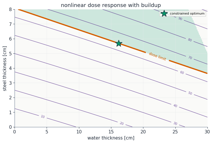
The orange curve is the dose limit. The feasible region is on the safe side of that curve. The purple curves are cost contours, and the optimizer is trying to find the lowest cost contour that still touches the feasible region.
The numerical coefficients are illustrative. The modeling lesson is real: dose constraints often come from attenuation and buildup calculations, and those constraints are usually easier to express first as physical requirements and then translate into solver form.
Example 3: A Linear Attenuation-Budget Model for linprog
Technical Specification
Now use a lower-fidelity shielding model. If we ignore thickness-dependent buildup, or reserve for it with a fixed conservative factor, the exponential attenuation model can be converted to a linear optical-thickness requirement:
where \(F\) is a fixed reserve factor. This is the same idea behind HVL/TVL budgeting: attenuation requirements are linear in shield thickness once we work in log transmission.
Water is cheap but bulky. Steel is compact but expensive. The design constraints are:
optical thickness supplied \(\ge \log(2D_0/D_{\max})\) using a fixed reserve factor of 2,
total thickness \(\le 35\) cm,
water thickness \(\le 30\) cm,
steel thickness \(\le 8\) cm,
nonnegative thicknesses.
Because the objective and all constraints are linear rows, this is a linprog problem. If the buildup factor varies with thickness, we are back in minimize territory.
[15]:
# Input block: linearized attenuation budget for the same shielding materials.
BUILDUP_RESERVE = 2.0
REQUIRED_TAU = np.log(BUILDUP_RESERVE*D0/D_LIMIT)
LP_TOTAL_THICKNESS = 35.0
LP_MAX_WATER = 30.0
LP_MAX_STEEL = 8.0
LP_COST = MATERIAL_COST

print("Input block")
print(f"fixed buildup reserve : {BUILDUP_RESERVE:.1f}")
print(f"required tau          : {REQUIRED_TAU:.3f}")
print(f"total thickness       : <= {LP_TOTAL_THICKNESS:.1f} cm")
print(f"water/steel limits    : water <= {LP_MAX_WATER:.1f} cm, steel <= {LP_MAX_STEEL:.1f} cm")
Input block
fixed buildup reserve : 2.0
required tau          : 4.605
total thickness       : <= 35.0 cm
water/steel limits    : water <= 30.0 cm, steel <= 8.0 cm
Translation to linprog
The attenuation row is a \(\ge\) constraint in the technical specification, but linprog wants \(\mathbf{A}_{ub}\mathbf{x} \le \mathbf{b}_{ub}\). Multiply that row by \(-1\).
The other engineering limits are already \(\le\) rows.
[16]:
# Translation block: linprog uses A_ub @ x <= b_ub, so >= rows must be multiplied by -1.
# Technical spec: MU[0]*water + MU[1]*steel >= REQUIRED_TAU
# linprog row:    -MU[0]*water - MU[1]*steel <= -REQUIRED_TAU
c_lp = LP_COST
A_ub_lp = np.array([
    [-MU[0], -MU[1]],  # attenuation budget >= REQUIRED_TAU
    [1.0, 1.0],        # total thickness <= LP_TOTAL_THICKNESS
    [1.0, 0.0],        # water thickness <= LP_MAX_WATER
    [0.0, 1.0],        # steel thickness <= LP_MAX_STEEL
])
b_ub_lp = np.array([
    -REQUIRED_TAU,
    LP_TOTAL_THICKNESS,
    LP_MAX_WATER,
    LP_MAX_STEEL,
])

row_names = ["attenuation", "total thickness", "water bound", "steel bound"]
print("linprog rows")
for name, row, rhs in zip(row_names, A_ub_lp, b_ub_lp):
    print(f"{name:16s}: {row} <= {rhs:.3f}")
linprog rows
attenuation     : [-0.086 -0.58 ] <= -4.605
total thickness : [1. 1.] <= 35.000
water bound     : [1. 0.] <= 30.000
steel bound     : [0. 1.] <= 8.000
[17]:
# Solve block.
lp_solution = linprog(
    c_lp,
    A_ub=A_ub_lp,
    b_ub=b_ub_lp,
    bounds=[(0.0, None), (0.0, None)],
    method="highs",
)

x_lp = lp_solution.x
active_lp = np.isclose(lp_solution.slack, 0.0, atol=1e-8)
[18]:
# Output/check block.
print("Output block")
print(f"success: {lp_solution.success}")
print(f"message: {lp_solution.message}")
print(f"water thickness = {x_lp[0]:.3f} cm")
print(f"steel thickness = {x_lp[1]:.3f} cm")
print(f"cost index      = {lp_solution.fun:.3f}")
print("slacks")
for name, slack, active in zip(row_names, lp_solution.slack, active_lp):
    print(f"  {name:16s}: slack={slack:8.3f}, active={active}")
print(f"tau supplied = {MU @ x_lp:.3f}")
Output block
success: True
message: Optimization terminated successfully. (HiGHS Status 7: Optimal)
water thickness = 30.000 cm
steel thickness = 3.492 cm
cost index      = 57.933
slacks
  attenuation     : slack=   0.000, active=True
  total thickness : slack=   1.508, active=False
  water bound     : slack=   0.000, active=True
  steel bound     : slack=   4.508, active=False
tau supplied = 4.605
[19]:
water = np.linspace(0.0, 35.0, 360)
steel = np.linspace(0.0, 8.5, 260)
W, S = np.meshgrid(water, steel)
feasible_lp = (
    (MU[0]*W + MU[1]*S >= REQUIRED_TAU)
    & (W + S <= LP_TOTAL_THICKNESS)
    & (W <= LP_MAX_WATER)
    & (S <= LP_MAX_STEEL)
)

fig, ax = plt.subplots(figsize=(7.2, 4.8), constrained_layout=True)
ax.contourf(W, S, feasible_lp, levels=[-0.5, 0.5, 1.5], colors=["white", COLORS["green"]], alpha=0.22)
ax.plot(water, (REQUIRED_TAU - MU[0]*water)/MU[1], color=COLORS["orange"], lw=2.6, label="attenuation requirement")
ax.plot(water, LP_TOTAL_THICKNESS - water, color=COLORS["muted"], lw=2.0, ls="--", label="total thickness")
ax.axvline(LP_MAX_WATER, color=COLORS["muted"], lw=2.0, ls=":", label="water limit")
ax.axhline(LP_MAX_STEEL, color=COLORS["muted"], lw=2.0, ls="-.", label="steel limit")
for level, alpha in [(45.0, 0.35), (lp_solution.fun, 0.9), (70.0, 0.35)]:
    ax.plot(water, (level - LP_COST[0]*water)/LP_COST[1], color=COLORS["purple"], lw=1.8, alpha=alpha)
ax.annotate("lower cost", xy=(28, 1.5), xytext=(21, 5.9),
            arrowprops={"arrowstyle": "->", "color": COLORS["purple"], "lw": 1.8},
            color=COLORS["purple"])
ax.plot(x_lp[0], x_lp[1], marker="*", ms=18, color=COLORS["green"], mec=COLORS["ink"], label="LP optimum")
ax.set_xlim(0, 35)
ax.set_ylim(0, 8.5)
ax.set_xlabel("water thickness [cm]")
ax.set_ylabel("steel thickness [cm]")
ax.set_title("linear log-attenuation model: cheap/bulky vs compact/expensive")
ax.legend(fontsize=8, loc="upper right")
style_axes(ax)
plt.show()
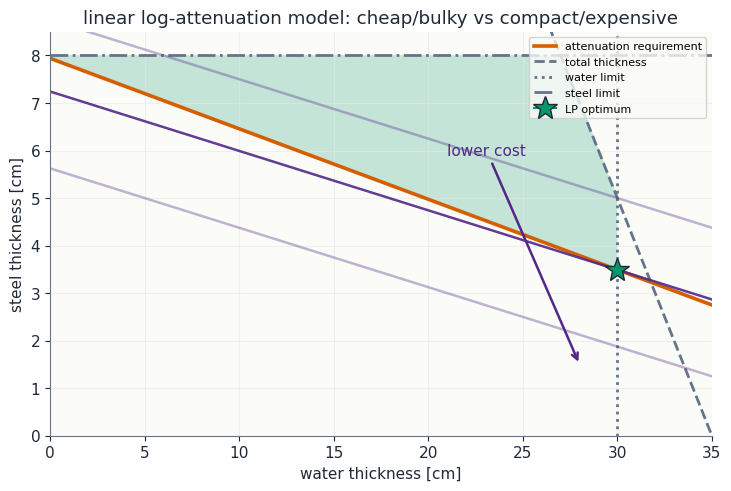
For a two-variable linear program, the picture is the lesson: the constraints carve out a polygon, and the objective line slides until it hits the last feasible corner. In higher dimensions the picture is harder to draw, but the bookkeeping idea is the same.
Here the LP approximation uses as much cheap water as allowed, then adds enough compact steel to meet the log-attenuation requirement. That is the competition the simplified model is resolving.
A Practical Decision Rule
If you can write the problem as rows of a matrix, use the row-based tool.
minimize: nonlinear objective, nonlinear constraints, simulation or model functions, curved feasible regions.linprog: linear objective, linear equality/inequality rows, bounds.
If you are unsure, start by writing down the variables and units. Then write the objective in one line. Then write each constraint as a sentence before translating it into code. A surprising number of optimization mistakes are translation mistakes, not algorithm mistakes.
Reading Solver Output
A useful solver result is not just the vector x. At minimum, inspect:
successandmessage,the objective value at the proposed optimum,
the constraint values at the proposed optimum,
active constraints, usually visible through near-zero slack,
whether the result changes when you try a reasonable different initial guess for nonlinear problems.
Do not report an optimization answer without a feasibility check. The number is not the answer until it has survived the check.
Further Reading
SciPy documentation for
`scipy.optimize.minimize<https://docs.scipy.org/doc/scipy/reference/generated/scipy.optimize.minimize.html>`__SciPy documentation for
`scipy.optimize.linprog<https://docs.scipy.org/doc/scipy/reference/generated/scipy.optimize.linprog.html>`__Shultis and Faw, Radiation Shielding, American Nuclear Society, for point-kernel shielding, attenuation, and buildup-factor context
Health Physics Society, Shielding of Gamma Radiation, for a compact discussion of buildup factors and shield-thickness calculations
NIST XCOM, X-Ray Mass Attenuation Coefficients, for attenuation data context
ANSI/ANS-6.4.3 material attenuation and buildup-factor data, and later revision work, for where engineering buildup-factor data come from
NRC, Regulatory Analysis Guidelines, and DOE, ALARA cost-benefit guide, for cost-dose trade-study context