Lesson 15 - Orthogonality, Gram–Schmidt, and Projection

Learning goals. By the end of this lecture, students will be able to:

• interpret dot products as both weighted sums and geometric measures of alignment,

• determine when vectors are orthogonal and explain why orthogonality is useful computationally,

• project one vector onto another vector or onto a subspace,

• construct an orthonormal basis using the Gram–Schmidt process,

• connect projections and orthonormal bases to least-squares approximation and model reduction ideas.

Key terms. orthogonality, projection, orthonormal basis, Gram–Schmidt process, least squares.

From operations to geometry

Lesson 11 introduced the dot product as a weighted sum,

\[\mathbf{u}^{\mathsf{T}}\mathbf{v}=\sum_{i=1}^n u_i v_i.\]

That interpretation is still important, but the dot product also carries geometric information. It tells us how much two vectors point in the same direction.

For nonzero vectors \(\mathbf{u}\) and \(\mathbf{v}\), the angle \(\theta\) between them satisfies

\[\mathbf{u}^{\mathsf{T}}\mathbf{v}=\left\lVert \mathbf{u} \right\rVert_2\left\lVert \mathbf{v} \right\rVert_2\cos\theta.\]

If the dot product is positive, the vectors point partly in the same direction. If it is negative, they point partly in opposite directions. If it is zero, the vectors are orthogonal.

Orthogonality

Two vectors are orthogonal if

\[\mathbf{u}^{\mathsf{T}}\mathbf{v}=0.\]

In two or three dimensions, orthogonality corresponds to a right angle. In higher dimensions, the picture is harder to draw, but the algebraic condition is the same.

Orthogonality is useful because independent contributions do not interfere. If \(\mathbf{u}\perp\mathbf{v}\), then

\[\left\lVert \mathbf{u}+\mathbf{v} \right\rVert_2^2=\left\lVert \mathbf{u} \right\rVert_2^2+\left\lVert \mathbf{v} \right\rVert_2^2.\]

This is the Pythagorean theorem in vector form.

A set of vectors \(\mathbf{q}_1,\ldots,\mathbf{q}_k\) is orthonormal if

\[\begin{split}\mathbf{q}_i^{\mathsf{T}}\mathbf{q}_j = \begin{cases} 1, & i=j,\\ 0, & i\neq j. \end{cases}\end{split}\]

If we collect these vectors as columns of a matrix

\[\mathbf{Q}=\begin{bmatrix}\mathbf{q}_1&\mathbf{q}_2&\cdots&\mathbf{q}_k\end{bmatrix},\]

then orthonormality is written compactly as

\[\mathbf{Q}^{\mathsf{T}}\mathbf{Q}=\mathbf{I}.\]

Projection onto a line

Suppose \(\mathbf{q}\) is a unit vector, meaning \(\left\lVert \mathbf{q} \right\rVert_2=1\). The projection of \(\mathbf{x}\) onto the line spanned by \(\mathbf{q}\) is

\[\widehat{\mathbf{x}}=(\mathbf{q}^{\mathsf{T}}\mathbf{x})\mathbf{q}.\]

The scalar \(\mathbf{q}^{\mathsf{T}}\mathbf{x}\) is the component of \(\mathbf{x}\) in the \(\mathbf{q}\) direction. Multiplying by \(\mathbf{q}\) turns that component back into a vector.

If the direction vector \(\mathbf{v}\) is not normalized, the projection is

\[\widehat{\mathbf{x}}=\frac{\mathbf{v}^{\mathsf{T}}\mathbf{x}}{\mathbf{v}^{\mathsf{T}}\mathbf{v}}\mathbf{v}.\]

The error \(\mathbf{x}-\widehat{\mathbf{x}}\) is orthogonal to the line:

\[\mathbf{v}^{\mathsf{T}}\left(\mathbf{x}-\widehat{\mathbf{x}}\right)=0.\]

This orthogonality condition is the key to least-squares problems.

The geometry is the important part. Projection splits one vector into a part the line can explain and a leftover part that points away from the line:

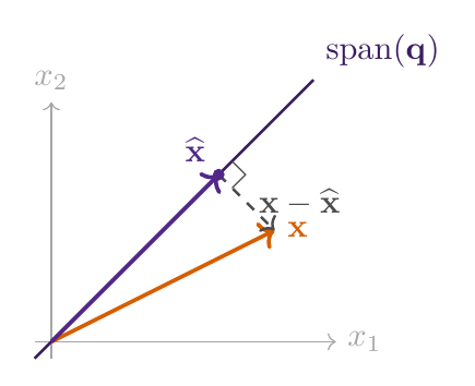
Figure. Projection onto a line decomposes \(\mathbf{x}\) into a component along the line and an orthogonal residual.

The formula matters because it computes the picture; the picture matters because it tells us what the formula is trying to do.

Example.

Let

\[\begin{split}\mathbf{x}=\begin{bmatrix}2\\1\end{bmatrix}, \qquad \mathbf{v}=\begin{bmatrix}1\\1\end{bmatrix}.\end{split}\]

Then

\[\begin{split}\widehat{\mathbf{x}} =\frac{\mathbf{v}^{\mathsf{T}}\mathbf{x}}{\mathbf{v}^{\mathsf{T}}\mathbf{v}}\mathbf{v} =\frac{3}{2}\begin{bmatrix}1\\1\end{bmatrix} =\begin{bmatrix}3/2\\3/2\end{bmatrix}.\end{split}\]

The error is

\[\begin{split}\mathbf{x}-\widehat{\mathbf{x}}=\begin{bmatrix}1/2\\-1/2\end{bmatrix},\end{split}\]

and this error is orthogonal to \(\mathbf{v}\).

Projection onto a subspace

A subspace is a flat set of vectors that is closed under linear combinations. A line through the origin is a one-dimensional subspace; a plane through the origin is a two-dimensional subspace. In higher dimensions the picture is harder to draw, but the rule is the same.

Let the columns of \(\mathbf{Q}\in\mathbb{R}^{n\times k}\) be an orthonormal basis for a subspace \(\mathcal{S}\). The orthogonal projection of \(\mathbf{x}\) onto \(\mathcal{S}\) is

\[\widehat{\mathbf{x}}=\mathbf{Q}\mathbf{Q}^{\mathsf{T}}\mathbf{x}.\]

The vector \(\mathbf{Q}^{\mathsf{T}}\mathbf{x}\) contains the coordinates of the projection in the orthonormal basis. Its entries are dot products:

\[\begin{split}\mathbf{Q}^{\mathsf{T}}\mathbf{x} = \begin{bmatrix} \mathbf{q}_1^{\mathsf{T}}\mathbf{x}\\ \mathbf{q}_2^{\mathsf{T}}\mathbf{x}\\ \vdots\\ \mathbf{q}_k^{\mathsf{T}}\mathbf{x} \end{bmatrix}.\end{split}\]

Multiplying by \(\mathbf{Q}\) converts those coordinates back to the original vector space:

\[\widehat{\mathbf{x}} =\mathbf{Q}\left(\mathbf{Q}^{\mathsf{T}}\mathbf{x}\right) =\sum_{i=1}^k \left(\mathbf{q}_i^{\mathsf{T}}\mathbf{x}\right)\mathbf{q}_i.\]

Figure. For orthonormal columns, \(\mathbf{Q}^{\mathsf{T}}\) measures coordinates by dot products and \(\mathbf{Q}\) reconstructs the projected vector from those coordinates.

The projection is the best approximation to \(\mathbf{x}\) from the subspace:

\[\widehat{\mathbf{x}}=\arg\min_{\mathbf{y}\in\mathcal{S}} \left\lVert \mathbf{x}-\mathbf{y} \right\rVert_2.\]

The error is orthogonal to the whole subspace:

\[\mathbf{Q}^{\mathsf{T}}\left(\mathbf{x}-\widehat{\mathbf{x}}\right)=\mathbf{0}.\]

This orthogonal-residual condition is the key idea to remember: projection is not only a formula, but the closest available approximation together with an error that points outside the chosen subspace.

If the basis columns in \(\mathbf{V}\) are linearly independent but not orthonormal, then the projection matrix is

\[\mathbf{V}\left(\mathbf{V}^{\mathsf{T}}\mathbf{V}\right)^{-1}\mathbf{V}^{\mathsf{T}}.\]

This formula is useful for interpretation, but it is usually less pleasant computationally than working with an orthonormal basis. If the columns are nearly dependent, \(\mathbf{V}^{\mathsf{T}}\mathbf{V}\) can be poorly conditioned, and the formula can magnify roundoff error.

Example.

A subspace projection with an orthonormal basis. Let

\[\begin{split}\mathbf{q}_1=\frac{1}{\sqrt{3}} \begin{bmatrix} 1\\1\\1 \end{bmatrix}, \qquad \mathbf{q}_2=\frac{1}{\sqrt{2}} \begin{bmatrix} -1\\0\\1 \end{bmatrix}.\end{split}\]

These vectors are orthonormal. If \(\mathbf{x}=[2,0,1]^T\), then the coordinates of the projection are

\[\mathbf{q}_1^{\mathsf{T}}\mathbf{x}=\sqrt{3}, \qquad \mathbf{q}_2^{\mathsf{T}}\mathbf{x}=-\frac{1}{\sqrt{2}}.\]

The projected vector is

\[\begin{split}\widehat{\mathbf{x}} =(\mathbf{q}_1^{\mathsf{T}}\mathbf{x})\mathbf{q}_1 +(\mathbf{q}_2^{\mathsf{T}}\mathbf{x})\mathbf{q}_2 = \begin{bmatrix} 3/2\\ 1\\ 1/2 \end{bmatrix}.\end{split}\]

The residual \(\mathbf{x}-\widehat{\mathbf{x}}=[1/2,-1,1/2]^T\) is orthogonal to both \(\mathbf{q}_1\) and \(\mathbf{q}_2\).

Least squares as projection

An overdetermined system

\[\mathbf{A}\mathbf{x}\approx\mathbf{b}\]

usually has more equations than unknowns. We cannot, in general, make \(\mathbf{A}\mathbf{x}\) equal \(\mathbf{b}\). Instead, least squares chooses \(\mathbf{x}\) to minimize the residual norm:

\[\mathbf{x}_{\text{ls}}=\arg\min_{\mathbf{x}}\left\lVert \mathbf{A}\mathbf{x}-\mathbf{b} \right\rVert_2.\]

Geometrically, \(\mathbf{A}\mathbf{x}_{\text{ls}}\) is the projection of \(\mathbf{b}\) onto the column space of \(\mathbf{A}\). Therefore, the residual

\[\mathbf{r}=\mathbf{b}-\mathbf{A}\mathbf{x}_{\text{ls}}\]

is orthogonal to every column of \(\mathbf{A}\). This gives the normal equations

\[\mathbf{A}^{\mathsf{T}}\mathbf{r}=\mathbf{0},\]

or

\[\mathbf{A}^{\mathsf{T}}\mathbf{A}\mathbf{x}_{\text{ls}}=\mathbf{A}^{\mathsf{T}}\mathbf{b}.\]

The normal equations are a compact way to express the projection condition. In practical numerical work, QR- or SVD-based algorithms are often preferred because they use orthonormal bases more directly and handle rank or conditioning issues more reliably.

Gram–Schmidt

Gram–Schmidt turns a linearly independent set of vectors into an orthonormal set spanning the same subspace. Suppose we start with \(\mathbf{v}_1,\ldots,\mathbf{v}_k\). The first basis vector is

\[\mathbf{q}_1=\frac{\mathbf{v}_1}{\left\lVert \mathbf{v}_1 \right\rVert_2}.\]

To build \(\mathbf{q}_2\), remove the component of \(\mathbf{v}_2\) in the \(\mathbf{q}_1\) direction:

\[\mathbf{w}_2=\mathbf{v}_2-(\mathbf{q}_1^{\mathsf{T}}\mathbf{v}_2)\mathbf{q}_1,\]

then normalize:

\[\mathbf{q}_2=\frac{\mathbf{w}_2}{\left\lVert \mathbf{w}_2 \right\rVert_2}.\]

The first nontrivial step is the same projection picture used in reverse. The candidate vector \(\mathbf{v}_2\) contains a part already explained by \(\mathbf{q}_1\). Gram–Schmidt subtracts that old part and keeps the new orthogonal direction.

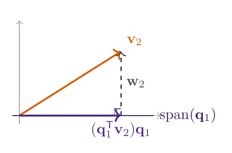
Figure. Gram–Schmidt removes the component already lying in the old direction, leaving a new vector orthogonal to that direction.

For the \(j\)th vector, subtract all previously constructed directions:

\[\mathbf{w}_j=\mathbf{v}_j-\sum_{i=1}^{j-1}(\mathbf{q}_i^{\mathsf{T}}\mathbf{v}_j)\mathbf{q}_i,\]

\[\mathbf{q}_j=\frac{\mathbf{w}_j}{\left\lVert \mathbf{w}_j \right\rVert_2}.\]

Algorithm.

Algorithm: Modified Gram–Schmidt

1. Start with linearly independent columns \(\mathbf{v}_1,\ldots,\mathbf{v}_k\).

2. For \(j=1,2,\ldots,k\), set \(\mathbf{w}=\mathbf{v}_j\).

3. For each previous basis vector \(\mathbf{q}_i\), subtract \((\mathbf{q}_i^{\mathsf{T}}\mathbf{w})\mathbf{q}_i\) from \(\mathbf{w}\).

4. Normalize the remaining vector: \(\mathbf{q}_j=\mathbf{w}/\left\lVert \mathbf{w} \right\rVert_2\).

Listing. Modified Gram–Schmidt in Python.

import numpy as np

def modified_gram_schmidt(V):
    V = V.astype(float)
    n, k = V.shape
    Q = np.zeros((n, k))
    R = np.zeros((k, k))
    for j in range(k):
        w = V[:, j].copy()
        for i in range(j):
            R[i, j] = Q[:, i] @ w
            w = w - R[i, j] * Q[:, i]
        R[j, j] = np.linalg.norm(w)
        if R[j, j] == 0.0:
            raise ValueError('dependent input vectors')
        Q[:, j] = w / R[j, j]
    return Q, R

The output satisfies approximately

\[\mathbf{Q}^{\mathsf{T}}\mathbf{Q}=\mathbf{I},\]

and

\[\mathbf{V}=\mathbf{Q}\mathbf{R}.\]

This is a QR factorization.

Example.

Discrete polynomial-like basis vectors. On the grid \(i=0,1,2,3\), start with the sampled monomials

\[\begin{split}\mathbf{v}_0= \begin{bmatrix} 1\\1\\1\\1 \end{bmatrix}, \qquad \mathbf{v}_1= \begin{bmatrix} 0\\1\\2\\3 \end{bmatrix}, \qquad \mathbf{v}_2= \begin{bmatrix} 0\\1\\4\\9 \end{bmatrix}.\end{split}\]

The first vector is the constant shape:

\[\begin{split}\mathbf{q}_0=\frac{1}{2} \begin{bmatrix} 1\\1\\1\\1 \end{bmatrix}.\end{split}\]

The component of \(\mathbf{v}_1\) along \(\mathbf{q}_0\) is

\[\mathbf{q}_0^{\mathsf{T}}\mathbf{v}_1=3,\]

so the centered linear part is

\[\begin{split}\mathbf{w}_1=\mathbf{v}_1-3\mathbf{q}_0= \begin{bmatrix} -3/2\\ -1/2\\ 1/2\\ 3/2 \end{bmatrix}.\end{split}\]

After normalization,

\[\begin{split}\mathbf{q}_1=\frac{1}{\sqrt{5}} \begin{bmatrix} -3/2\\ -1/2\\ 1/2\\ 3/2 \end{bmatrix}.\end{split}\]

For the quadratic sample, remove the constant and linear parts:

\[\begin{split}\mathbf{w}_2 = \mathbf{v}_2 -(\mathbf{q}_0^{\mathsf{T}}\mathbf{v}_2)\mathbf{q}_0 -(\mathbf{q}_1^{\mathsf{T}}\mathbf{v}_2)\mathbf{q}_1 = \begin{bmatrix} 1\\-1\\-1\\1 \end{bmatrix},\end{split}\]

so

\[\begin{split}\mathbf{q}_2=\frac{1}{2} \begin{bmatrix} 1\\-1\\-1\\1 \end{bmatrix}.\end{split}\]

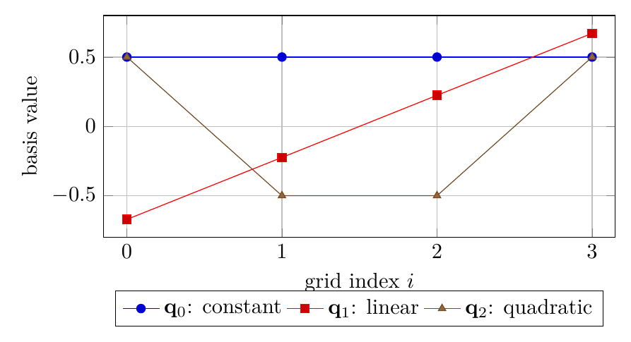
Figure. A discrete constant-linear-quadratic orthonormal basis on four sample points. The scale is less important than the shapes and their orthogonality.

This is a discrete analogue of building orthogonal polynomials: begin with simple powers of the grid index, then remove what has already been represented. A sampled response can then be reconstructed from basis coefficients. For example, if

\[\begin{split}\mathbf{x}= \begin{bmatrix} 2\\2\\3\\5 \end{bmatrix},\end{split}\]

then

\[\mathbf{q}_0^{\mathsf{T}}\mathbf{x}=6, \qquad \mathbf{q}_1^{\mathsf{T}}\mathbf{x}=\sqrt{5}, \qquad \mathbf{q}_2^{\mathsf{T}}\mathbf{x}=1,\]

and the reconstruction is

\[\mathbf{x} = 6\mathbf{q}_0+\sqrt{5}\mathbf{q}_1+\mathbf{q}_2.\]

The three coefficients say how much constant, linear, and quadratic shape is present in this four-point signal.

Why orthonormal bases are computationally useful

If \(\mathbf{Q}\) has orthonormal columns, then projecting onto its column space is simple:

\[\widehat{\mathbf{x}}=\mathbf{Q}\mathbf{Q}^{\mathsf{T}}\mathbf{x}.\]

Coordinates are computed by dot products:

\[\mathbf{c}=\mathbf{Q}^{\mathsf{T}}\mathbf{x}.\]

Lengths are preserved under square orthogonal transformations:

\[\left\lVert \mathbf{Q}\mathbf{z} \right\rVert_2=\left\lVert \mathbf{z} \right\rVert_2\]

when \(\mathbf{Q}^{\mathsf{T}}\mathbf{Q}=\mathbf{I}\) and \(\mathbf{Q}\) is square. These properties make orthonormal bases stable and convenient in least squares, model reduction, and iterative methods.

Example.

A Galerkin system from a projection condition. Suppose we want an approximate solution of \(\mathbf{A}\mathbf{x}=\mathbf{b}\) in the two-dimensional subspace spanned by the orthonormal columns of \(\mathbf{Q}\). We write

\[\mathbf{x}\approx \mathbf{Q}\mathbf{y}.\]

The residual is

\[\mathbf{r}=\mathbf{b}-\mathbf{A}\mathbf{Q}\mathbf{y}.\]

A Galerkin condition asks that this residual be orthogonal to the same subspace:

\[\mathbf{Q}^{\mathsf{T}}\mathbf{r}=\mathbf{0}.\]

Substituting the residual gives the smaller system

\[\mathbf{Q}^{\mathsf{T}}\mathbf{A}\mathbf{Q}\mathbf{y} = \mathbf{Q}^{\mathsf{T}}\mathbf{b}.\]

This system did not come out of thin air: it is the orthogonality condition applied to the residual. Krylov and finite-element methods use this same projection logic with more carefully chosen subspaces.

Connection to Krylov ideas

Lesson 14 ended with repeated matrix-vector products. There, the iteration index \(k\) was a sweep or generation counter: Richardson, Jacobi, and Gauss–Seidel repeatedly converted a residual into a new population estimate, mostly keeping only the current iterate. Krylov methods keep more of that generated history. Starting from a residual \(\mathbf{r}_0\), one can build the sequence

\[\mathbf{r}_0,\quad \mathbf{A}\mathbf{r}_0,\quad \mathbf{A}^2\mathbf{r}_0,\quad \ldots\]

The span of the first \(k\) vectors is a Krylov subspace:

\[\mathcal{K}_k(\mathbf{A},\mathbf{r}_0)=\operatorname{span}\{\mathbf{r}_0,\mathbf{A}\mathbf{r}_0,\ldots,\mathbf{A}^{k-1}\mathbf{r}_0\}.\]

The vectors in this sequence can become nearly dependent, so orthonormalization is essential in many Krylov methods. Gram–Schmidt applied to this sequence is the core idea behind Arnoldi iteration, GMRES, and related algorithms.

We will not develop GMRES fully here. The important message for this course is that the same ingredients keep appearing:

\[\text{matrix-vector products} + \text{orthogonality} + \text{projection}.\]

Connection to eigenvectors

Orthogonality also appears in eigenvalue problems. For real symmetric matrices, eigenvectors associated with distinct eigenvalues are orthogonal. This is one reason symmetric eigenvalue problems are especially well behaved.

Power iteration in Lesson 16 repeatedly multiplies by \(\mathbf{A}\) and normalizes. More advanced eigenvalue algorithms keep several directions at once, orthogonalize them, and project the matrix onto a lower-dimensional subspace. The geometry in this chapter is therefore not separate from eigenvalue computation; it is one of the foundations.

Exercises

1. Let \(\mathbf{u}=[1,2,-1]^T\) and \(\mathbf{v}=[2,-1,0]^T\). Compute \(\mathbf{u}\cdot\mathbf{v}\). Are the vectors orthogonal?

2. Project \(\mathbf{x}=[2,1]^T\) onto the line spanned by \(\mathbf{v}=[1,1]^T\). What is the projection error, and how can you check that it is orthogonal to \(\mathbf{v}\)?

3. Apply the first two steps of Gram–Schmidt to \(\mathbf{v}_1=[1,1,0]^T\) and \(\mathbf{v}_2=[1,0,1]^T\). Give \(\mathbf{q}_1\) and \(\mathbf{q}_2\).

4. Explain why orthonormal columns make projection and coordinate calculations easier.

Answers.

1. The dot product is \(1(2)+2(-1)+(-1)(0)=0\), so the vectors are orthogonal.

2. The projection coefficient is \(3/2\), so

   \[\begin{split}\widehat{\mathbf{x}}= \frac{3}{2} \begin{bmatrix} 1\\ 1 \end{bmatrix} = \begin{bmatrix} 3/2\\ 3/2 \end{bmatrix}.\end{split}\]

The error is \([1/2,-1/2]^T\), and its dot product with \([1,1]^T\) is zero.

1. The first vector is

   \[\begin{split}\mathbf{q}_1=\frac{1}{\sqrt{2}} \begin{bmatrix} 1\\ 1\\ 0 \end{bmatrix}.\end{split}\]

Subtracting the part of \(\mathbf{v}_2\) along \(\mathbf{q}_1\) gives

\[\begin{split}\mathbf{w}_2= \begin{bmatrix} 1/2\\ -1/2\\ 1 \end{bmatrix}, \qquad \mathbf{q}_2=\frac{1}{\sqrt{6}} \begin{bmatrix} 1\\ -1\\ 2 \end{bmatrix}.\end{split}\]

1. If \(\mathbf{Q}\) has orthonormal columns, coordinates are \(\mathbf{Q}^T\mathbf{x}\), and the projection is \(\mathbf{Q}\mathbf{Q}^T\mathbf{x}\). No normal-equation solve is needed.

End-of-lecture summary

Takeaway.

• The dot product measures both weighted sums and geometric alignment.

• Orthogonal vectors have zero dot product and independent length contributions.

• Projection gives the closest vector in a line or subspace, and the projection error is orthogonal to that subspace.

• Least squares is a projection problem onto a column space.

• Gram–Schmidt builds an orthonormal basis from independent vectors.

• Orthonormal bases support stable projections, least-squares solves, Krylov methods, and eigenvalue algorithms.