Lesson 14 - Norms, Sparse Matrices, and Iterative Methods

Learning goals. By the end of this lecture, students will be able to:

• compute and interpret common vector norms as measures of magnitude, error, and residual size,

• use residuals such as \(\mathbf{r}=\mathbf{b}-\mathbf{A}\mathbf{x}\) to assess an approximate linear-system solution,

• explain why sparse matrices are useful for large engineering models,

• store and multiply sparse matrices using SciPy tools,

• describe iterative methods as repeated matrix-vector products plus corrections,

• compare Richardson, Jacobi, and Gauss–Seidel as residual-correction rules with different local information flow,

• connect fixed-point convergence to repeated error multiplication and the spectral radius of an iteration matrix,

• explain why forming \(\mathbf{A}^{-1}\) is usually avoided.

Key terms. vector norm, residual norm, sparse matrix, matrix-vector product, fixed-point iteration, preconditioner, Jacobi iteration, Gauss–Seidel iteration, spectral radius.

The basic question

At this point in the course, we know how to assemble systems and solve small ones directly. Now suppose someone hands us a matrix \(\mathbf{A}\), a right-hand side \(\mathbf{b}\), and a candidate solution \(\mathbf{x}\). Before we ask whether it is beautiful, fast, or physically interesting, the first question is simpler:

\[\text{Does } \mathbf{A}\mathbf{x}=\mathbf{b}\text{?}\]

The computable answer is the residual

\[\mathbf{r}=\mathbf{b}-\mathbf{A}\mathbf{x}.\]

If \(\mathbf{r}=\mathbf{0}\), the equations are satisfied exactly. More generally, the residual lives in equation space: it is the balance defect left after substituting a candidate \(\mathbf{x}\) into the original equations. In a transport balance, it is leftover source, removal, and scattering bookkeeping. In floating-point arithmetic and in iterative methods, we usually ask whether this leftover is small enough.

This raises a second question: what does “small” mean for a vector?

Vector norms

That word “small” needs a meter. A vector norm maps a vector to a nonnegative scalar that measures its size. For \(1\leq p < \infty\), the general \(p\)-norm is

\[\left\lVert \mathbf{v} \right\rVert_p = \left(\sum_{i=1}^n |v_i|^p\right)^{1/p}.\]

The limit case \(p=\infty\) keeps only the largest component:

\[\left\lVert \mathbf{v} \right\rVert_{\infty} = \max_i |v_i|.\]

The \(1\)- and \(2\)-norms are the two common finite cases used in this lesson:

\[\left\lVert \mathbf{v} \right\rVert_1 = \sum_{i=1}^n |v_i|.\]

\[\left\lVert \mathbf{v} \right\rVert_2 = \left(\sum_{i=1}^n v_i^2\right)^{1/2}.\]

The \(1\)-norm measures total absolute magnitude. The \(2\)-norm is the Euclidean length. The \(\infty\)-norm measures the largest component.

For residuals, a typical absolute stopping criterion is

\[\left\lVert \mathbf{r}^{(k)} \right\rVert_2 < \text{tolerance}.\]

A typical relative stopping criterion is

\[\frac{\left\lVert \mathbf{r}^{(k)} \right\rVert_2}{\left\lVert \mathbf{b} \right\rVert_2} < \text{tolerance}.\]

The relative form asks whether the balance defect is small compared with the scale of the data.

Listing. Computing common vector norms.

import numpy as np

v = np.array([2.0, -3.0, 6.0])
print(np.linalg.norm(v, 1))
print(np.linalg.norm(v, 2))
print(np.linalg.norm(v, np.inf))

11.0
7.0
6.0

Example.

One vector, three different summaries. For \(\mathbf{v}=[2,-3,6]^T\),

\[\left\lVert \mathbf{v} \right\rVert_1=11, \qquad \left\lVert \mathbf{v} \right\rVert_2=7, \qquad \left\lVert \mathbf{v} \right\rVert_\infty=6.\]

All three statements are true, but they answer different questions. The \(1\)-norm reports total absolute magnitude, the \(2\)-norm reports Euclidean length, and the \(\infty\)-norm reports the largest component. When reporting a residual vector, choose the norm that matches the interpretation.

Residual versus error

Let \(\mathbf{x}^{\ast}\) be the exact solution of

\[\mathbf{A}\mathbf{x}^{\ast}=\mathbf{b}.\]

The error in an approximate solution \(\mathbf{x}^{(k)}\) is

\[\mathbf{e}^{(k)}=\mathbf{x}^{\ast}-\mathbf{x}^{(k)}.\]

The residual is

\[\begin{split}\begin{aligned} \mathbf{r}^{(k)} &= \mathbf{b}-\mathbf{A}\mathbf{x}^{(k)} \\ &= \mathbf{A}\mathbf{x}^{\ast}-\mathbf{A}\mathbf{x}^{(k)} \\ &= \mathbf{A}\mathbf{e}^{(k)}. \end{aligned}\end{split}\]

So the residual is not the same thing as the error, but it is connected to the error. If \(\mathbf{A}\) is invertible,

\[\mathbf{e}^{(k)}=\mathbf{A}^{-1}\mathbf{r}^{(k)}.\]

Taking norms gives the bound

\[\left\lVert \mathbf{e}^{(k)} \right\rVert \leq \left\lVert \mathbf{A}^{-1} \right\rVert\,\left\lVert \mathbf{r}^{(k)} \right\rVert.\]

The matrix norm here measures amplification: it asks how much \(\mathbf{A}^{-1}\) can stretch a residual when we translate it back into an error. This is the part worth slowing down for. Residuals measure leftover equation imbalance, while errors measure distance from the true unknown vector. A small residual is good evidence that the equations are nearly satisfied; it is not, by itself, a certificate that the unknown vector is close to the exact one. The problem’s scaling and conditioning still matter. For iterative methods, the residual history also needs context: a residual that decreases slowly may be warning us about an error-propagation matrix with eigenvalues close to one in magnitude.

\[\begin{split}\begin{array}{ccccc} \text{solution space} & \mathbf{e}^{(k)} & \xrightarrow{\ \mathbf{A}\ } & \mathbf{r}^{(k)} & \text{equation space}\\ \text{distance from } \mathbf{x}^{\ast} & & & \text{leftover balance defect} \end{array}\end{split}\]

Takeaway.

The residual is computable because it uses \(\mathbf{A}\), \(\mathbf{b}\), and the candidate solution. The true error usually is not computable because the exact solution is unknown.

Example.

A small residual can still hide an amplified error. Let

\[\begin{split}\mathbf{A}= \begin{bmatrix} 1 & 0\\ 0 & 10^{-3} \end{bmatrix}, \qquad \mathbf{x}^{\ast}= \begin{bmatrix} 1\\ 1 \end{bmatrix}, \qquad \mathbf{x}= \begin{bmatrix} 1\\ 0 \end{bmatrix}.\end{split}\]

The error is \(\mathbf{e}=[0,1]^T\), but the residual is

\[\begin{split}\mathbf{r}=\mathbf{A}\mathbf{e}= \begin{bmatrix} 0\\ 10^{-3} \end{bmatrix}.\end{split}\]

Thus the residual 2-norm is \(10^{-3}\), while the error 2-norm is \(1\). The residual is still useful, but it must be interpreted through the conditioning and scaling of the operator.

\[\begin{split}\begin{bmatrix} 0\\ 10^{-3} \end{bmatrix} \xrightarrow{\ \mathbf{A}^{-1}\ } \begin{bmatrix} 0\\ 1 \end{bmatrix}.\end{split}\]

In this example, a small residual component in equation space becomes a large error component in solution space.

Why sparsity appears

The next question is where the matrix came from. Large engineering matrices are often mostly zero, and those zeros are not decoration. They usually come from locality. In a one-dimensional nearest-neighbor transport model, a neutron that leaves cell \(i\) can move only to nearby cells during one step, so the equation for cell \(i\) involves only cell \(i\) and its two Cartesian neighbors:

\[x_{i-1} \longrightarrow x_i \longleftarrow x_{i+1}.\]

That local movement becomes a narrow sparse band in the matrix:

\[\begin{split}\mathbf{A}=\begin{bmatrix} 1 & -c/2 & 0 & \cdots & 0\\ -c/2 & 1 & -c/2 & \ddots & \vdots\\ 0 & -c/2 & 1 & \ddots & 0\\ \vdots & \ddots & \ddots & \ddots & -c/2\\ 0 & \cdots & 0 & -c/2 & 1 \end{bmatrix}.\end{split}\]

Only about \(3n\) entries are nonzero, even though the dense matrix has \(n^2\) entries.

The same idea extends to Cartesian grids. A two-dimensional cell \((i,j)\) has a five-point stencil, and a three-dimensional cell \((i,j,k)\) has a seven-point stencil:

\[\begin{split}\begin{aligned} \text{2-D:}\quad &(i,j),\ (i-1,j),\ (i+1,j),\ (i,j-1),\ (i,j+1),\\ \text{3-D:}\quad &(i,j,k),\ (i\pm 1,j,k),\ (i,j\pm 1,k),\ (i,j,k\pm 1). \end{aligned}\end{split}\]

The stencil is the local picture of one matrix row: the row for a cell has nonzeros only for the cell itself and the neighbors that directly enter its balance.

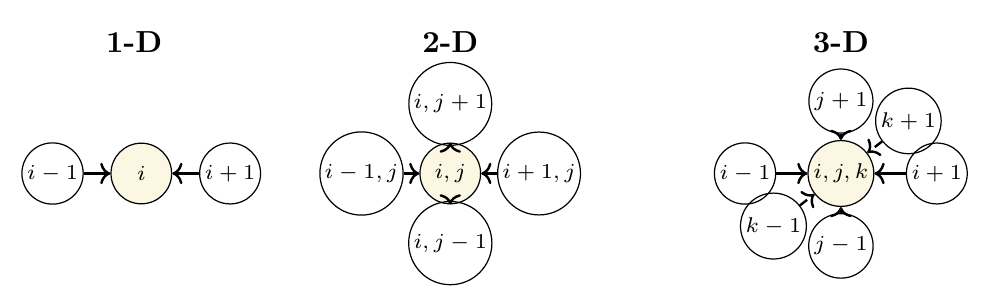
Figure. Cartesian nearest-neighbor stencils. The highlighted unknown is updated from itself and only the adjacent cells that share a face with it.

A spy plot shows the same local rule after all cells have been flattened into one vector. If a dot marks a stored nonzero, the one-dimensional nearest-neighbor matrix looks like

\[\begin{split}\operatorname{spy}(\mathbf{A})\approx \begin{bmatrix} \bullet & \bullet & & & \\ \bullet & \bullet & \bullet& & \\ & \bullet & \bullet& \bullet& \\ & & \ddots & \ddots & \ddots \\ & & & \bullet& \bullet \end{bmatrix}.\end{split}\]

This is the locality assumption made visible: most cell pairs do not talk directly in one step. The two- and three-dimensional matrices have more bands and blocks, but they are still sparse because each row has only a handful of neighbor entries.

For a dense \(n\times n\) matrix, storage costs \(O(n^2)\), and a matrix-vector product costs \(O(n^2)\). For a sparse matrix with \(\text{nnz}\) stored nonzeros, storage costs \(O(\text{nnz})\), and a sparse matrix-vector product costs approximately \(O(\text{nnz})\). For nearest-neighbor Cartesian grids, the stencil size stays small: about \(3n\) entries in one dimension, \(5n\) in two dimensions, and \(7n\) in three dimensions, up to boundary corrections.

Example.

Counting what locality saves. For \(n=10{,}000\) unknowns, a dense matrix has \(10^8\) entries. A tridiagonal nearest-neighbor matrix has about \(3n=30{,}000\) stored entries. A five-point stencil on a two-dimensional grid has about \(5n=50{,}000\) stored entries. The exact boundary count is not the point: locality changes the storage story from quadratic to essentially linear in the number of unknowns.

Sparse matrices in SciPy

SciPy provides sparse matrix formats. Coordinate form is the most direct starting point: store the row index, column index, and value for each nonzero entry. That is the location-value version of the matrix picture above. It is also a natural construction format when an engineering model loops over cells, elements, or interactions and drops one contribution at a time into the global operator.

Listing. Building a sparse matrix from coordinate triples.

import numpy as np
import scipy.sparse as sp

n = 5
c = 0.9
rows, cols, data = [], [], []
for i in range(n):
    rows.append(i); cols.append(i); data.append(1.0)
    if i > 0:
        rows.append(i); cols.append(i-1); data.append(-c/2)
    if i < n-1:
        rows.append(i); cols.append(i+1); data.append(-c/2)

A_coo = sp.coo_matrix((data, (rows, cols)), shape=(n, n))
A = A_coo.tocsr()

Coordinate form is not always the fastest format for repeated operations, but it is often the simplest way to assemble the matrix. After assembly, we usually convert to a format better matched to the next operation. Two common formats are:

• CSR, or compressed sparse row, which is efficient for row access and matrix-vector products,

• CSC, or compressed sparse column, which is often used by sparse direct solvers and factorizations.

The older Python for Engineers sparse-systems examples used small tridiagonal matrices to make the same point visually: a handful of bands can represent the whole operator. A plot of the nonzero pattern is often more informative than printing a large matrix. For visual work, keep the example small enough that the stencil structure is visible.

Listing. Building small Cartesian nearest-neighbor matrices.

c = 0.9

def cartesian_neighbor_matrix(shape, c=0.9):
    """Nearest-neighbor Cartesian balance matrix for a small grid."""
    rows, cols, data = [], [], []
    ndim = len(shape)
    neighbor_weight = -c / (2 * ndim)
    for cell in np.ndindex(shape):
        row = np.ravel_multi_index(cell, shape)
        rows.append(row); cols.append(row); data.append(1.0)
        for axis in range(ndim):
            for step in (-1, 1):
                nbr = list(cell)
                nbr[axis] += step
                if 0 <= nbr[axis] < shape[axis]:
                    rows.append(row)
                    cols.append(np.ravel_multi_index(tuple(nbr), shape))
                    data.append(neighbor_weight)
    n = int(np.prod(shape))
    return sp.coo_matrix((data, (rows, cols)), shape=(n, n)).tocsr()

A_1d = cartesian_neighbor_matrix((8,), c)
A_2d = cartesian_neighbor_matrix((4, 4), c)
A_3d = cartesian_neighbor_matrix((3, 3, 3), c)
A = A_1d

for name, mat in [("1-D", A_1d), ("2-D", A_2d), ("3-D", A_3d)]:
    print(name, mat.shape, "nnz =", mat.nnz)

1-D (8, 8) nnz = 22
2-D (16, 16) nnz = 64
3-D (27, 27) nnz = 135

The attribute A.nnz reports the number of stored nonzero entries. This is often a more meaningful measure of problem size than \(n^2\) for sparse models.

Listing. Seeing 1-D, 2-D, and 3-D locality with spy plots.

import matplotlib.pyplot as plt

fig, axes = plt.subplots(1, 3, figsize=(10.5, 3.2), constrained_layout=True)
for ax, mat, title, markersize in zip(
    axes,
    [A_1d, A_2d, A_3d],
    ["1-D line: 3-point stencil", "2-D grid: 5-point stencil", "3-D grid: 7-point stencil"],
    [10, 6, 4],
):
    ax.spy(mat, markersize=markersize)
    ax.set_title(title)
    ax.set_xlabel("column")
    ax.set_ylabel("row")

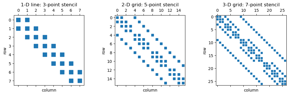
The plot marks only stored nonzeros. The 1-D case is tridiagonal. The 2-D case has a block pattern because each row of the grid talks to its left, right, up, and down neighbors. The 3-D case adds another layer of block structure for the \(z\)-neighbors. In the video version of this lesson, plt.spy is the visual anchor: it turns the modeling assumption “only nearby cells interact during one step” into a pattern students can see before they think about storage formats.

Direct solves and fill-in

A sparse direct solve often factors the matrix. Conceptually, this is still related to the LU factorization from Lesson 12. However, factorization can create new nonzero entries in \(\mathbf{L}\) and \(\mathbf{U}\) that were zero in \(\mathbf{A}\). This is called fill-in.

For one-dimensional tridiagonal problems, fill-in is mild. For large two- or three-dimensional models, fill-in can be substantial. This is one reason sparse direct methods can become expensive even when the original matrix is sparse.

For this lesson, fill-in is a warning rather than a new algorithmic topic. We will use sparse direct solves as a reliable check on small examples, but we will not build the full machinery of sparse factorization or reordering here.

Never form the inverse

The notation

\[\mathbf{x}=\mathbf{A}^{-1}\mathbf{b}\]

is mathematically convenient, but it is usually a poor computational plan. Even if \(\mathbf{A}\) is sparse, \(\mathbf{A}^{-1}\) is typically dense. Forming it can use far more memory than the original model and can be less stable than solving systems directly.

In this course, the practical rule is:

\[\text{solve } \mathbf{A}\mathbf{x}=\mathbf{b}; \qquad \text{do not explicitly compute } \mathbf{A}^{-1}\text{ unless there is a special reason.}\]

This rule also matters for eigenvalue algorithms. Inverse iteration in Lesson 16 uses solves with \(\mathbf{A}\), not an explicitly formed inverse.

From physics to fixed-point iteration

Return to the random-walk model. The steady equation can be written as

\[\mathbf{x}=\mathbf{b}+c\mathbf{P}\mathbf{x},\]

where \(\mathbf{P}\) moves population to neighboring cells and \(c\) is the scattering ratio. This suggests a fixed-point iteration:

\[\mathbf{x}^{(k+1)}=\mathbf{b}+c\mathbf{P}\mathbf{x}^{(k)}.\]

Starting from \(\mathbf{x}^{(0)}=\mathbf{0}\), each step adds the source and scatters the previous population.

The superscript \(k\) is a sweep or generation index for the whole population vector. It is time-like, but it is not the clock for one particle history. This connects back to Monte Carlo simulation habits: when particle histories are given a common time origin, we can compare population that belongs to the same generation or tally window across cells. Here \(\mathbf{x}^{(k)}\) is the population after \(k\) source-plus-scatter layers have been accumulated, and \(\mathbf{x}^{(k+1)}\) adds one more layer.

If we define

\[\mathbf{A}=\mathbf{I}-c\mathbf{P},\]

then the steady equation is

\[\mathbf{A}\mathbf{x}=\mathbf{b}.\]

Now ask what the residual buys us if we do not want to factor \(\mathbf{A}\). For this splitting, the fixed-point update becomes

\[\begin{split}\begin{aligned} \mathbf{x}^{(k+1)} &= \mathbf{b}+c\mathbf{P}\mathbf{x}^{(k)} \\ &= \mathbf{x}^{(k)}+\left(\mathbf{b}-\mathbf{A}\mathbf{x}^{(k)}\right) \\ &= \mathbf{x}^{(k)}+\mathbf{r}^{(k)}. \end{aligned}\end{split}\]

This is Richardson iteration with step size one.

This is also the geometric-series intuition behind source iteration. Each step adds one more scattered contribution. When \(c\) is small, later histories shrink quickly. When \(c\) is close to one, neutrons survive more scattering events, the memory of earlier errors persists longer, and the residual can decay slowly.

Listing. Richardson iteration using sparse matrix-vector products.

def richardson(A, b, kmax=100):
    x = np.zeros_like(b)
    residual_norms = []
    for k in range(kmax):
        r = b - A @ x
        residual_norms.append(np.linalg.norm(r))
        x = x + r
    return x, np.array(residual_norms)

Each iteration uses a sparse matrix-vector product and vector additions. No factorization is required.

Jacobi and Gauss–Seidel as corrected residual updates

Richardson iteration uses the residual directly. More generally, we can apply an inexpensive approximate inverse to the residual:

\[\mathbf{x}^{(k+1)}=\mathbf{x}^{(k)}+\mathbf{M}^{-1}\left(\mathbf{b}-\mathbf{A}\mathbf{x}^{(k)}\right).\]

Here \(\mathbf{M}\) is a preconditioner: a useful choice is inexpensive to solve with and approximates \(\mathbf{A}\) well enough to improve convergence. This \(M\) is separate from the random-walk matrix \(P\) used earlier in the transport model.

For this discussion, split the matrix into three pieces:

\[\mathbf{A}=\mathbf{D}+\mathbf{L}+\mathbf{U}.\]

Here \(\mathbf{D}\) contains only the diagonal entries, \(\mathbf{L}\) is the strictly lower-triangular part, and \(\mathbf{U}\) is the strictly upper-triangular part. The word strictly matters: \(\mathbf{L}\) and \(\mathbf{U}\) do not include the diagonal.

\[\begin{split}\operatorname{spy}(\mathbf{D})\approx \begin{bmatrix} \bullet& & \\ &\bullet& \\ & &\bullet \end{bmatrix}, \qquad \operatorname{spy}(\mathbf{L})\approx \begin{bmatrix} & & \\ \bullet& & \\ &\bullet& \end{bmatrix}, \qquad \operatorname{spy}(\mathbf{U})\approx \begin{bmatrix} &\bullet& \\ & &\bullet\\ & & \end{bmatrix}.\end{split}\]

If \(\mathbf{M}=\mathbf{D}\), the diagonal of \(\mathbf{A}\), the method is Jacobi iteration:

\[\mathbf{x}^{(k+1)}=\mathbf{x}^{(k)}+\mathbf{D}^{-1}\mathbf{r}^{(k)}.\]

This updates each unknown using old neighbor values. For the tridiagonal nearest-neighbor model above, an interior-cell update has the form

\[x_i^{(k+1)} = b_i+\frac{c}{2}x_{i-1}^{(k)} +\frac{c}{2}x_{i+1}^{(k)}.\]

Every cell in the new layer is computed from the same old layer \(k\), so Jacobi has a clean parallel picture:

\[\begin{array}{ccccc} x_{i-1}^{(k)} & \longrightarrow & x_i^{(k+1)} & \longleftarrow & x_{i+1}^{(k)} . \end{array}\]

If \(\mathbf{M}=\mathbf{D}+\mathbf{L}\), where \(\mathbf{L}\) is the strictly lower-triangular part of \(\mathbf{A}\), the method is Gauss–Seidel iteration:

\[\mathbf{x}^{(k+1)}=\mathbf{x}^{(k)}+(\mathbf{D}+\mathbf{L})^{-1}\mathbf{r}^{(k)}.\]

This corresponds to sweeping through the unknowns and using new values as soon as they are available. For a left-to-right sweep through the same nearest-neighbor model,

\[x_i^{(k+1)} = b_i+\frac{c}{2}x_{i-1}^{(k+1)} +\frac{c}{2}x_{i+1}^{(k)}.\]

The left neighbor has already been updated during the current sweep, while the right neighbor is still from the old layer:

\[\begin{array}{ccccc} x_{i-1}^{(k+1)} & \longrightarrow & x_i^{(k+1)} & \longleftarrow & x_{i+1}^{(k)} . \end{array}\]

The index \(k\) is still an algorithmic generation or sweep index. Gauss–Seidel changes how information travels inside that sweep; it does not turn the solve into a literal physical particle clock.

The three methods can be viewed through their preconditioner patterns. Using the small one-dimensional matrix from the spy example keeps the diagonal, strictly lower, and strictly upper parts visible:

Listing. Seeing correction rules with spy plots.

A_split = A_1d
D = sp.diags(A_split.diagonal(), format="csr")
L = sp.tril(A_split, k=-1, format="csr")
U = sp.triu(A_split, k=1, format="csr")

fig, axes = plt.subplots(1, 4, figsize=(11, 3), constrained_layout=True)
for ax, mat, title in zip(
    axes,
    [D, L, U, D + L],
    ["D: diagonal", "L: strictly lower", "U: strictly upper", "Gauss-Seidel: D + L"],
):
    ax.spy(mat, markersize=10)
    ax.set_title(title)

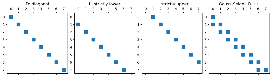
The picture is the Python for Engineers matrix-splitting story rewritten as residual correction. Richardson applies the residual directly, Jacobi uses a local diagonal scale, and Gauss–Seidel uses the diagonal plus the strictly lower part for a left-to-right sweep. The strictly upper part contains neighbor information that has not yet been updated during that sweep.

Convergence as error multiplication

A stationary iteration has the form

\[\mathbf{x}^{(k+1)}=\mathbf{G}\mathbf{x}^{(k)}+\mathbf{g}.\]

If \(\mathbf{x}^{\ast}\) is the fixed point, then the error satisfies

\[\mathbf{e}^{(k+1)}=\mathbf{G}\mathbf{e}^{(k)}.\]

Thus convergence depends on repeated multiplication by \(\mathbf{G}\). This observation leads directly to the eigenvalue discussion in Lesson 16. For now, the important point is that an iterative method converges only if its error-propagation matrix damps all error components.

The spectral radius summarizes this damping:

\[\rho(\mathbf{G})=\max_i |\lambda_i(\mathbf{G})|.\]

For this lesson, read this as a preview rather than a new eigenvalue task. For a basic stationary iteration, \(\rho(\mathbf{G})<1\) means repeated error multiplication tends to damp the error. If \(\rho(\mathbf{G})\) is close to one, convergence may happen, but it will often be slow. Lesson 16 develops the eigenvalue machinery more directly.

For source iteration,

\[\mathbf{G}=c\mathbf{P}.\]

For a finite domain with boundary leakage, \(\rho(\mathbf{P})\) is usually below one because some population leaves the modeled system. Larger \(c\) and less leakage push \(\rho(\mathbf{G})\) closer to one, so population survives more scattering events and convergence can be slow. This physical interpretation matches the numerical behavior because \(c\) directly scales the source-iteration error-propagation matrix.

Example.

Two Richardson steps as accumulated scattering. Starting from \(\mathbf{x}^{(0)}=\mathbf{0}\),

\[\begin{split}\begin{aligned} \mathbf{x}^{(1)} &= \mathbf{b},\\ \mathbf{x}^{(2)} &= \mathbf{b}+c\mathbf{P}\mathbf{b},\\ \mathbf{x}^{(3)} &= \mathbf{b}+c\mathbf{P}\mathbf{b}+c^2\mathbf{P}^2\mathbf{b}. \end{aligned}\end{split}\]

The iteration is not mysterious: each step adds one more layer of scattered contribution. This is also why the method can be slow when \(c\) is near one. Many scattering histories remain important, so many iterations may be required before the residual becomes small.

Why this leads to subspaces

Stationary methods use a fixed rule and typically remember only the current iterate. If convergence is slow, it is natural to ask whether we can keep more information. For example, we might keep the current residual, the previous residual, and other directions generated by repeated matrix-vector products.

That idea leads to subspace methods. Before discussing them, we need geometry: dot products, orthogonality, projections, and orthonormal bases. Those are the topics of Lesson 15.

Exercises

1. Let \(\mathbf{v}=[2,-1,2]^T\). Compute \(\left\lVert \mathbf{v} \right\rVert_1\), \(\left\lVert \mathbf{v} \right\rVert_2\), and \(\left\lVert \mathbf{v} \right\rVert_\infty\).

2. Let

   \[\begin{split}\mathbf{A}= \begin{bmatrix} 4 & -1\\ -1 & 3 \end{bmatrix}, \qquad \mathbf{x}= \begin{bmatrix} 1\\ 1 \end{bmatrix}, \qquad \mathbf{b}= \begin{bmatrix} 2\\ 5 \end{bmatrix}.\end{split}\]

Compute the residual \(\mathbf{r}=\mathbf{b}-\mathbf{A}\mathbf{x}\) and its infinity norm.

1. A five-point stencil is assembled on a \(100\times 100\) grid. Give a rough upper bound for the number of nonzeros and compare it with the number of entries in a dense matrix of the same size.

2. For a stationary iteration \(\mathbf{x}^{(k+1)}=\mathbf{G}\mathbf{x}^{(k)}+\mathbf{g}\), explain why convergence depends on repeated multiplication by \(\mathbf{G}\).

Answers.

1. The norms are

   \[\left\lVert \mathbf{v} \right\rVert_1=5,\qquad \left\lVert \mathbf{v} \right\rVert_2=3,\qquad \left\lVert \mathbf{v} \right\rVert_\infty=2.\]

2. Since \(\mathbf{A}\mathbf{x}=[3,2]^T\), the residual is

   \[\begin{split}\mathbf{r}= \begin{bmatrix} -1\\ 3 \end{bmatrix}, \qquad \left\lVert \mathbf{r} \right\rVert_\infty=3.\end{split}\]

3. There are \(n=10{,}000\) unknowns. A five-point stencil has at most about \(5n=50{,}000\) nonzeros, while a dense matrix would have \(n^2=100{,}000{,}000\) entries.

4. If \(\mathbf{x}^\ast\) is the fixed point, the error satisfies \(\mathbf{e}^{(k+1)}=\mathbf{G}\mathbf{e}^{(k)}\). The iteration converges only if repeated multiplication by \(\mathbf{G}\) damps every error component.

End-of-lecture summary

Takeaway.

• Norms turn vector residuals and errors into scalar measures of size.

• The residual is computable; the true error usually is not.

• Sparse matrices store and operate only on nonzero entries, which can reduce memory and cost dramatically.

• Sparse direct methods can suffer from fill-in, and explicit inverses are usually dense.

• Iterative methods repeatedly apply matrix-vector products and corrections.

• Convergence of stationary iteration is governed by repeated multiplication of the error by an iteration matrix, setting up the eigenvalue ideas in Lesson 16.