Numerical Solutions of First-Order Systems

Overview, Objectives, and Key Terms

This lesson is a direct extension of the last lesson, in which the focus was the numerical solution of first-order IVPs. Here, those techniques are extended to systems of first-order equations.

Objectives

By the end of this lesson, you should be able to

• Set up and solve simple linear systems numerically using NumPy.
• Solve systems of first-order IVPs numerically using forward and backward Euler’s method
• Solve systems of first-order IVPs using odeint

Prerequisites

You should already be able to

• Solve IVPs using Euler’s method (forward and backward)
• Define one- and two-dimensional arrays using NumPy arrays
• Use np.linalg.solve to solve \(\mathbf{Ax = b}\)

Please review these topics (and resources) as needed.

Key Terms

• odeint
• first-order system

A Coupled System and Its Numerical Solution

Let’s motivate the discussion with the familiar spring-mass system:

\[m \frac{d^2 x}{dt^2} = -k x - a \frac{dx}{dt} \, ,\]

subject to subject to the ICs \(x(0) = x_0\) and \(x'(0) = v_0\). This equation can be solved directly as a second-order equation using standard techniques or by using SymPy. It would also be possible to solve this numerically by applying the appropriate finite-difference approximations to both \(d^x/dt^2\) and \(dx/dt\). There are a variety of ways to do this (we have more than one way to approximate \(y'\) for instance), and each would be somewhat more complicated than the Euler methods previously discussed.

Instead, we reduce the second-order problem to a system of two first-order problems. Let

\[\frac{dx}{dt} = v(t)\]

from which we have

\[\frac{dv}{dt} = -\frac{kx(t) + av(t)}{m} \, .\]

These two equations can be written more compactly in matrix form:

\[\begin{split}\left [ \begin{array}{c} v' \\ x' \end{array} \right ] = \left [ \begin{array}{cc} -\frac{a}{m} & -\frac{k}{m} \\ 1 & 0 \\ \end{array} \right ] \left [ \begin{array}{c} v(t) \\ x(t) \end{array} \right ]\end{split}\]

or

\[\mathbf{y}' = \mathbf{A}\mathbf{y}(t) \, ,\]

where \(\mathbf{y} = [v(t), x(t)]^T\) and \(T\) is the transpose.

By writing the system in this form, it can be observed to follow the more general form

\[\mathbf{y}' = \mathbf{f}(t, \mathbf{y}(t)) \, ,\]

for which the forward Euler method is defined as

\[\mathbf{y}(t_{n+1}) = \mathbf{y}(t_n) + \Delta \mathbf{f}(t, \mathbf{y}(t_n)) \, ,\]

where \(t_{n+1} = t_{n} + \Delta\). The simplicity of forward Euler is obvious here: no matter how complicated \(\mathbf{f}\) might be, all we need to do is evaluate it once using information defined at the old time \(t_n\) to determine the solution at the new time \(t_{n+1}\). It’s explicit. We do not need to solve any linear or nonlinear systems. For the case of the spring-mass systems, that step looks like

\[\mathbf{y}(t_{n+1}) = \mathbf{y}(t_n) + \Delta \mathbf{A} \mathbf{y}(t_n) \, .\]

---

Exercise: Consider the spring-mass system. For \(m = 1\), \(k = 1\), \(a = 1\), \(x(0) = 0\), and \(v(0) = 1\), compute \(x(t)\) at \(t = [0, 0.5, 1.0, \ldots, 10]\) (that’s 21 times) using forward Euler. Plot these estimates and the actual solution.

Solution: First, let’s get the reference solution using SymPy in the form of a callable, lambdified function. For completeness, return both \(x(t)\) and \(v(t)\):

def spring_mass_reference(m, k, a, x_0, v_0):
    # set up symbols
    import sympy as sy
    x, t = sy.symbols('x t')
    # set up/solve IVP
    ivp = sy.Eq(m*sy.diff(x(t), t, 2), -k*x(t) - a*sy.diff(x(t), t))
    sol = sy.dsolve(ivp)
    # set up/solve ICs
    ic1 = sy.Eq(sol.rhs.subs(t, 0), x_0)
    ic2 = sy.Eq(sy.diff(sol.rhs, t, 1).subs(t, 0), v_0)
    coefs = sy.solve([ic1, ic2], [sy.Symbol('C1'), sy.Symbol('C2')])
    # make substitutions and return the lambdified results
    sol_x = sol.rhs.subs(coefs).simplify()
    sol_v = sy.diff(sol_x, t)
    f_x = sy.lambdify(t, sol_x)
    f_v = sy.lambdify(t, sol_v)
    return f_v, f_x

Now, apply forward Euler.

import numpy as np
# Define givens
m, k, a, x0, v0 = 1, 1, 1, 0, 1
# Define the times
t = np.linspace(0, 10, 21)
# Define the solution and set the ICs
y_fe = np.zeros((len(t), 2))
y_fe[0, 0] = v0
y_fe[0, 1] = x0
# Define the 2 by 2 matrix A.  Note the spacing
# used to enhance readability.
A = np.array([[-a/m, -k/m],
              [1,    0   ]])
# Define the time step
Delta = t[1] - t[0]
# Now, loop through for each time step
for i in range(0, len(t)-1):
    y_fe[i+1] = y_fe[i] + Delta*A.dot(y_fe[i])
# Extract v and x.
v_fe, x_fe = y_fe[:, 0], y_fe[:, 1]
# Get the reference values (as functions)
v_ref, x_ref = spring_mass_reference(m, k, a, x0, v0)
# Plot
import matplotlib.pyplot as plt
plt.plot(t, x_fe, 'k-o', t, x_ref(t), 'r--o')
plt.xlabel('t')
plt.ylabel('x(t)')
plt.legend(['approx', 'actual'])
plt.show()

---

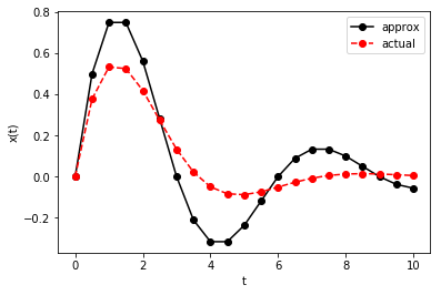
Exercise: This numerical solution for the spring-mass equation above is qualitatively close to the reference found using SymPy, but it’s quantitatively far enough away that I’m suspicious. Compute the absolute error in \(x(10)\) as a function of \(\Delta\). Does it converge?

---

Exercise: An important phenomenon in nuclear reactors is the production of \({}^{135}\)Xe, a substance that is really good at absorbing the neutrons needed to sustain the chain reaction that powers such reactors. \({}^{135}\)Xe is produced directly from fission, but it is also generated from the decay of \({}^{135}\)I, another nuclide produced by fission. Details aside, the concentrations of these nuclides is well modeled by the following system of equations:

\[\frac{d N_{I}}{dt} = \gamma_{I} \Sigma_f \phi - \lambda_I N_I(t) \, ,\]

and

\[\frac{d N_{Xe}}{dt} = \gamma_{Xe} \Sigma_f \phi + \lambda_I N_I(t) - \sigma_a^{Xe} N_{Xe}(t) \phi + \lambda_{Xe} N_{Xe}(t) \, .\]

Suppose that \(\sigma_a^{Xe} = 3.5 \times 10^{-18}\) cm\(^2\), \(\gamma_{Xe} = 0.006\), \(\gamma_I = 0.064\), \(\lambda_{Xe} = 2.95\times 10^{-5}\) 1/s, and \(\lambda_{I} = 2.1\times 10^{-5}\) 1/s, and \(\Sigma_f = 0.1\) 1/cm. s.

1. If \(\phi\) has units of 1/cm\(^2\), what is the unit of \(N_I\) and \(N_{Xe}\)?
2. Find the steady-state (i.e., equilibrium) value of \(N_I\) and \(N_{Xe}\) when \(\phi = 10^{14}\) 1/cm\(^2\). Remember, steady state means “constant in time.” Hence, set the derivatives to zero, and solve for \(N^{SS}_I\) and \(N^{SS}_{Xe}\).
3. Use those steady-state values \(N^{SS}_I\) and \(N^{SS}_{Xe}\) as the initial condition for the IVP at \(t = 0\). Solve the equations using forward Euler for \(\phi = 10^{13}\) 1/cm\(^2\), \(\phi = 10^{14}\) 1/cm\(^2\), and \(\phi = 2\times 10^{14}\) 1/cm\(^2\) for times up 24 hours. (Be careful about the step size you use.)

---

When the Equations are “Stiff”

A system of IVPs is considered “stiff” when the underlying time constants vary by several orders of magnitude. That means one part of the solution (one nuclide, or the position of one mass in a spring-mass system) may grow or decay exponentially over periods of seconds, whereas some other part of the solution may vary over much smaller time periods, e.g., ms or smaller. Forward Euler fails for these systems unless \(\Delta\) is very, very small. Sometimes, it must be small enough that solving the system becomes impractical.

An alternative is to use methods that are implicit in time. The chief example is backward Euler. Remember, implicit here means the solution at \(t_{n+1}\) depends on information at \(t_{n+1}\), not \(t_{n}\). For systems of IVPs, we need to solve a matrix system to make the step. For nonlinear IVPs, we need to solve a nonlinear equation (perhaps a system) to make the step.

Let’s go back to the generic equation

\[\mathbf{y}' = \mathbf{f}(t, \mathbf{y}(t)) \, .\]

Application of backward Euler gives

\[\mathbf{y}(t_{n+1}) = \mathbf{y}(t_n) + \Delta \mathbf{f}(t_{n+1}, \mathbf{y}(t_{n+1})) \,\]

where, again, \(t_{n+1} = t_{n} + \Delta\). For the case of the spring-mass systems, this backward-Euler step looks like

\[\mathbf{y}(t_{n+1}) = \mathbf{y}(t_n) + \Delta \mathbf{A} \mathbf{y}(t_{n+1}) \, .\]

Note that \(\mathbf{y}(t_{n+1})\) is on both sides of the equation. To isolate it, we move the right-most term to the left-hand side, which leads to

\[(\mathbf{I} - \Delta \mathbf{A}) \mathbf{y}(t_{n+1}) = \mathbf{y}(t_n) \, .\]

This is a linear equation of the form \(\mathbf{Mx}=\mathbf{b}\), and we can use numpy.linalg.solve to solve such systems.

---

Exercise: Solve the system \(x + 2y = 3\) and \(2x - y = 2\) for \(x\) and \(y\) using numpy.

Solution: First, recognize this is the same as the matrix equation

\[\begin{split}\left [ \begin{array}{cc} 1 & 2 \\ 2 & -1 \\ \end{array} \right ] \left [ \begin{array}{c} x \\ y \end{array} \right ] = \left [ \begin{array}{c} 3 \\ 2 \end{array} \right ]\end{split}\]

Then, set up this matrix and vector using numpy arrays, and solve using numpy.linalg.solve:

M = np.array([[1,  2],
              [2, -1]])
b = np.array([3, 2])
v = np.linalg.solve(M, b)
x, y = v
x, y

(1.3999999999999999, 0.80000000000000004)

One can also check the answer makes sense. Here, we should get \(\mathbf{b}\) from the matrix-vector product \(\mathbf{Mv}\):

M.dot(v)

array([ 3.,  2.])

---

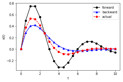
Example Solve the spring-mass example from above using backward Euler.

Solution:

# We already have all the values set.  We'll
# make a new solution array to compare BE to
# FE and the reference.

# Define the solution and set the ICs
y_be = np.zeros((len(t), 2))
y_be [0, 0] = v0
y_be [0, 1] = x0

# Make the 2x2 identity
I = np.eye(2)

# Now, loop through for each time step
for i in range(0, len(t)-1):
    y_be[i+1] = np.linalg.solve(I-Delta*A, y_be[i])

# Extract v and x.
v_be, x_be = y_be[:, 0], y_be[:, 1]

# Plot
plt.plot(t, x_fe, 'k-o', t, x_be, 'b-^', t, x_ref(t), 'r--o')
plt.xlabel('t')
plt.ylabel('x(t)')
plt.legend(['forward', 'backward', 'actual'])
plt.show()

---

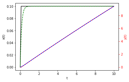
Example: For \(\Delta = 0.1\), compute \(x(10)\) and \(y(10)\) by solving the following system using (1) forward Euler and (2) backward Euler:

\[\begin{split}\left [ \begin{array}{c} x' \\ y' \end{array} \right ] = \left [ \begin{array}{rr} -10 & 0.00 \\ 10 & -0.01 \\ \end{array} \right ] \left [ \begin{array}{c} x(t) \\ y(t) \end{array} \right ] + \left [ \begin{array}{c} 1 \\ 0 \end{array} \right ]\end{split}\]

for \(x(0) = y(0) = 0\). How do things change when \(\Delta = 0.2\)? \(\Delta = 0.001\)?

Solution:

t = np.linspace(0, 10, 101)
z_fe = np.zeros((len(t), 2))
z_be = np.zeros((len(t), 2))
A = np.array([[-10,  0.00],
              [10,  -0.01]])
s = np.array([1, 0])
I = np.eye(2)
Delta = t[1]-t[0]
for i in range(0, len(t)-1):
    z_fe[i+1] = z_fe[i] + Delta*(A.dot(z_fe[i]) + s)
    z_be[i+1] = np.linalg.solve(I-Delta*A, z_be[i] + Delta*s)

fig, ax1 = plt.subplots()
ax1.plot(t, z_fe[:, 0], 'k', t, z_be[:, 0], 'g--')
ax1.set_xlabel('t')
ax1.set_ylabel('x(t)', color='k')
ax1.tick_params('y', colors='k')
ax2 = ax1.twinx()
ax2.plot(t, z_fe[:, 1], 'r', t, z_be[:, 1], 'b--')
ax2.set_ylabel('y(t)', color='r')
ax2.tick_params('y', colors='r')
plt.show()

SciPy’s odeint

While the Euler methods are proven and simple techniques for solving first-order IVPs, routine analysis is best performed using more robust methods like those implemented in SciPy’s odeint. The basic ingredients needed to solve an IVP with odeint are a function that represents \(y'\), the times at which \(y(t)\) is to be evaluated, and the initial conditions.

Specifically, the scipy.integrate.odeint function is used to solve individual, first-order IVP’s or systems of such equations. Behind the scenes, either an Adams or BDF method is used depending on the behavior of the solution. All of this is automatic, and more details can be found in the documentation.

Use of odeint For A Single IVP

Let’s revisit our single IVP example, namely \(y' + y(t) = 2\) with \(y(0)=1\) for \(t\in [0, 10]\). The odeint function requires, at a minimum, three inputs: (1) a function that evaluates the derivative \(y'(t)\) given the time \(t\) and the value of the function \(f(t)\), (2) the initial condition \(y(0)=y_0\), and (3) the times at which \(y(t)\) is to be evaluated. These times are independent of the times and corresponding \(\Delta\)‘s used internally; they only are used for the output.

The derivative function has two arguments: the time \(t\) at which \(y'\) is to be evaluated, and the value of \(y\) at that same time. That sounds like you need to know \(y(t)\) beforehand—but you don’t! This derivative function is only called behind the scenes by odeint itself. Hence, odeint knows (or has an approximation to) \(y\) at the time \(t\), and your job is to use the two to define \(y'\). For our example, that means we need a function that evaluates and returns

\[\frac{dy}{dt} = 2 - y(t) \, .\]

With that, we can implement a complete odeint solution to our example:

import numpy as np
import matplotlib.pyplot as plt
from scipy.integrate import odeint

# derivative function
def y_prime(y, t) :
    return 2.0 - y

# times at which y(t) is to be evaluated
times = np.linspace(0, 10)

# exact solution
y_exact = 2 - np.exp(-times)

# solve with odeint
y_odeint = odeint(y_prime, y0=1.0, t=times)

plt.plot(times, y_odeint, 'k', times, y_exact, 'ro')
plt.legend(['$y_{\\mathrm{odeint}}$', '$y_{\\mathrm{exact}}$'], loc=0, numpoints = 1)
plt.show()

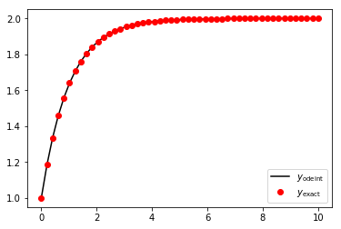
The odeint result is very good, with no discernible error (to my eyes, anyway). We can plot the errors, but first we need to reshape the output from odeint. Notice that it has an explicit, 2-D shape, whereas y_exact yields a 1-D array (from the 1-D t_odeint):

print(y_odeint.shape)
print(y_exact.shape)
print(times.shape)

(50, 1)
(50,)
(50,)

Normally, this apparent mismatch is no big deal—we plotted both against the same t_odeint array. However, the mismatch does lead to strange results when we try to compute the error. The solution, however, is to make them the same size, and we can do that, e.g., with an explicit reshaping:

y_odeint_reshaped = y_odeint.reshape((len(times),))
error = y_odeint_reshaped - y_exact
print(error.shape)

(50,)

plt.plot(times, error, 'r-o')
plt.xlabel('t')
plt.ylabel('$y_{\\mathrm{odeint}}-y_{\\mathrm{exact}}$')
plt.show()

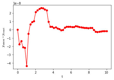
Two features of this error warrant discussion. First, the overall magnitude of the odeint error is smaller than the errors we previously found using \(N=100\) with forward Euler. Second, the error fluctuates more than we found for forward Euler and is more uniform in magnitude. The overall magnitude of the error is determined by the desired numerical accuracy (defined by the optional arguments rtol and atol). The time-dependent fluctuations are due to use of nonuniform time steps. The details are well beyond our scope, but you’ll recall from the Taylor expansion of \(y'\) that the errors are related to \(y''\). If some estimate can be made of \(y''\) during the time-stepping procedure, then the error can also be estimated. Proper selection of \(\Delta\) (either larger or smaller) can yield errors just within the desired tolerance, ensuring proper accuracy and avoiding use of too many small steps in regions where they are not needed. This all happens automatically within odeint.

---

Exercise: Solve the following IVPs using odeint and plot the result for \(t \in [0, 5]\):

1. \(\frac{dy}{dt} = e^{-y}\) for \(y(0) = 0\).
2. \(\frac{dy}{dt} = x^2 + y^2\) for \(y(0) = 1\).
3. \(\frac{dy}{dt} = y - y^2\) for \(y(0) = 0.5\).

---

Use of odeint for Systems of IVPs

The same ingredients needed for solving one IVP with odeint are needed for systems. Now, however, the right-hand side function returns multiple values for each unknown.

---

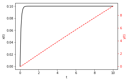
Exercise: Solve

\[\begin{split}\left [ \begin{array}{c} x' \\ y' \end{array} \right ] = \left [ \begin{array}{rr} -10 & 0.00 \\ 10 & -0.01 \\ \end{array} \right ] \left [ \begin{array}{c} x(t) \\ y(t) \end{array} \right ] + \left [ \begin{array}{c} 1 \\ 0 \end{array} \right ]\end{split}\]

for \(x(0) = y(0) = 0\) and \(t \in [0, 10]\) using odeint fo

Solution: First, import odeint:

from scipy.integrate import odeint

Then, define the derivative function. Here, that’s everything on the right-hand side of the original IVP.

def derivative(z, t):
    """ Evaluate the right-hand side of the IVP.  Here, t
        is the time at which things are evaluated, and
        z = [x, y] is the solution at that time.
    """
    A = np.array([[-10, 0],
                  [10, -0.01]])
    z_prime = A.dot(z) + np.array([1, 0])
    return z_prime

Define the times and solve the problem:

t = np.linspace(0, 10, 100)
ic = [0, 0]
z = odeint(derivative, ic, t)

Finally, plot the result.

fig, ax1 = plt.subplots()
ax1.plot(t, z[:, 0], 'k-') # Note z[:, 0], NOT z[0, :]
ax1.set_xlabel('t')
ax1.set_ylabel('x(t)', color='k')
ax1.tick_params('y', colors='k')
ax2 = ax1.twinx()
ax2.plot(t, z[:, 1], 'r--')
ax2.set_ylabel('y(t)', color='r')
ax2.tick_params('y', colors='r')
plt.show()

---

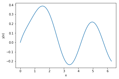
Exercise: Consider the second-order equation for damped, harmonic motion:

\[y'' + 2y'+2y=\sin(2x)\]

for \(y(0)=0\) and \(y'(0)=0.5\). Solve this using odeint for \(t \in [0, 2\pi]\).

Solution: This is second order, so we need to convert it first into a system of first-order equations. Let \(y' = v\). Then, \(v' = \sin(2x) - 2v - 2y\). Now, implement this as a derivative function:

def derivative(z, x):
    y, v = z  # unpacking and computing
    yp = v    # y' and v' separately
    vp = np.sin(2*x) - 2*v - 2*y
    return [yp, vp] # lists are fine

Set the times, ICs, and solve:

x = np.linspace(0, 2*np.pi, 100)
ic = [0, 0.5]
# this is another way to get the individual
# solution components:
y, v = odeint(derivative, ic, x).T
plt.plot(x, y)
plt.xlabel('x')
plt.ylabel('y(x)')
plt.show()

Further Reading

Make sure you know how to use odeint for single equations and systems of equations. A good resource to supplement this lesson is the odeint documentation and any examples include therein.