Lecture 26 - Solving ODEs Symbolically¶

Overview, Objectives, and Key Terms¶

In this lecture, we revisit the tools provided by SymPy and apply them to solution of ordinary differential equations (ODEs). Engineering is full of ODEs, since they are fundamental to the language of balance relationships found in heat transfer, nuclear reactor physics, control systems, and other areas. The goal here is not to present the theory of ODEs, nor is it to present the various systematic ways be which one can determine solutions to ODEs. Rather, the focus is placed squarely on defining ODEs symbolically, solving them symbolically, and, importantly, applying initial or boundary conditions to those symbolic solutions and solving the resulting algebraic equations for any undetermined coefficients. In other words, the focus is on the problem solving process.

Objectives¶

By the end of this lesson, you should be able to

Define first- and second-order, ordinary differential equations symbolically
Solve first- and second-order, ODEs symbollically
Apply initial and boundary conditions as is appropriate to determine complete solutions to ODEs important in engineering disciplines.

Prerequisites¶

You should already be able to

Solve ODEs based on what you’ve learned in a course like MATH 340 (this is not a strict requirement, but if you have not had MATH 340, you may wish to set up a time with me or the TAs).
Set up and solve algebraic systems using SymPy
Perform subsitution into symbolic values using SymPy
Define derivatives of arbitrary functions using SymPy

Key Terms¶

differential equation
ordinary
linear
ODE
initial value problem
boundary value problem

Differential Equations¶

A differential equation is any equation in which an unknown function $f$ appears with one of more of its derivatives. When $f$ is a function of only one variable, the derivatives are ordinary (as opposed to partial), and the equation is an ordinary differential equation (ODE). In compact notation, such an equation may be written

\[\begin{equation} \mathcal{L}f(x) = q(x) \, , \end{equation}\]

where $\mathcal{L}$ is a differential operator. If $\mathcal{L}$ contains only linear combinations of $f(x)$ and its derivates, then $\mathcal{L}$ is a linear operator, and the equation is a linear ODE. If $q(x) = 0$, the equation is homogeneous and is otherwise inhomogeneous. If the highest derivative of $f(x)$ present in $\mathcal{L}f$ is $n$ (i.e., $d^n f/dx^n$), then the equation is called an nth-order equation.

Examples of linear operators include $\mathcal{L}f = \frac{df}{dx}$ and $\mathcal{L}f = a(x) \frac{d^2f}{dx^2} + b(x)$, where $a(x)$ and $b(x)$ are arbitrary functions of $x$ (but not of $f(x)$). For comparison, a nonlinear example is $\mathcal{L}f = \left ( \frac{df}{dx} \right )^2 - \sqrt{f(x)}$, which includes nonlinear functions of $f$ and its first derivative.

Our focus in this and the next module is entirely on linear, ordinary differential equations and their solution by symbolic and numerical techniques.

Whence Comes $y'+py=q$?¶

For now, we’ll keep it simple and consider problems of the form

\[\begin{equation} \frac{dy}{dt} + p(t)y(t) = q(t) \, , \qquad y(0) = y_0 \, . \end{equation}\]

This is a first-order, initial-value problem (IVP). It is first order because there is only a first derivative. It is an initial-value problem because the unknown (here, $y(t)$) is specified at some “initial” time.

A first-order IVP can be used to represent of a number of physical phenomena. The first that comes to mind (to me, as a nuclear engineer) is radioactive decay with external production, usually written $N' = -\lambda N(t) + R(t)$, where $N(t)$ is the number of radioactive nuclei at time $t$, $\lambda$ is the decay constant (with units of inverse seconds), and $R(t)$ is the number of new nuclei born per second. The time rate of change of $N(t)$ is a balance of those new nuclei from $R(t)$ against the number $-\lambda N(t)$ lost by decay. For sufficiently long times, $dy/dt \to 0$, and $y = R/\lambda$, a steady state in which losses are exactly balanced by gains.

An equally good example is the case of an object of mass $m$ in free fall through a viscuous medium, e.g., the atmosphere. If some object is held a distance above the earth and dropped, its acceleration at any point in time is related to the net forces acting on the body. These forces include the gravitational force $F_g = -m g$ (i.e., downward) and the air resistance $F_r$. A simple resistance model is $F_r = cv$, where $c$ is a (positive) constant and $v$ is the velocity directed toward Earth. Hence, the downward force is

\[\begin{equation} F(t) = -cv(t) + m g \, . \end{equation}\]

From Newton’s second law, $F = ma$, so we have

\[\begin{equation} ma(t) = m \frac{dv}{dt} = -cv(t) + mg \, , \end{equation}\]

or

\[\begin{equation} v' = -\frac{c}{m} v(t) + g \, . \end{equation}\]

The positive $c/m$ has the same effect as a positive $\lambda$ in radioactive decay: the larger the velocity $v$, the larger the retardation force $cv$ (just like the larger the number of nuclei $N$, the larger the number $\lambda N$ decaying per unit time). For the free-fall case, the steady-state condition $v'=0$ has a special name: terminal velocity.

Lots of phenomena have this sort of behavior, this natural negative feedback, and such feedback can help us when we solve these problems numerically. In those cases where the feedback is positive, we expect the number of nuclei to grow more and more (or, equivalent, for a falling object to keep accelerating toward earth). The former happens when pythons (or neutrons) multiply in nature; thankfully, the hail of northeastern Kansas does reach a terminal velocity. Oh, and I’m not joking about pythons: combine the Malthusian model with the fact there is an artificial source term due to pet owners releasing their larger-than-expected pets into the Florida Everglades.

Symbolic Solution of First-Order IVPs¶

By “Hand”¶

First, a sanity check $\frac{dy}{dt} = ay(t)$ with $y(0) = y_0$. This can be solved, and it depends on only integration. Rearrange the equation to be

\[\frac{1}{y}dy = a dt \, ,\]

and then integrate to obtain

\[\ln(y) = a t + C' \, .\]

Here, $C'$ is an arbitrary integration constant. Exponentiation of both sides results in

\[y(t) = e^{at + C'} = C e^{at} \, ,\]

where $C = e^{C'}$ is still an arbitrary constant.

So far, this is just integral calculus. To solve the given IVP, we need to apply the initial condition (IC). Specifically, we need to specify $C$ that satisfies $y(0) = C e^{a0} = y_0$. Clearly, $C = y_0$.

With SymPy¶

With this simplest of IVPs solved “by hand,” we turn to SymPy and its dsolve function. First, initialize the symbols:

In [1]:

import sympy as sy
sy.init_printing()
y, y_0, a, t = sy.symbols('y y_0 a t')

Then, set up the differential equation just like any other equation:

In [2]:

ivp = sy.Eq(sy.diff(y(t), t), a*y(t))
ivp

Out[2]:

\[$$\frac{d}{d t} y{\left (t \right )} = a y{\left (t \right )}$$\]

Finally, produce the general solution via

In [3]:

sol = sy.dsolve(ivp)
sol

Out[3]:

\[$$y{\left (t \right )} = C_{1} e^{a t}$$\]

The solution returned is a SymPy equation (i.e., sy.Eq) relating $y(t)$ on the left-hand side to $C_1 e^{at}$ on the right-hand side. We want to get the right-hand side and determine $C_1$ given the initial condition. To do so, we can use the rhs attribute of sy.Eq:

In [4]:

sol.rhs

Out[4]:

\[$$C_{1} e^{a t}$$\]

In [5]:

C = sy.solve(sy.Eq(sol.rhs.subs(t, 0), y_0), sy.Symbol('C1'))
C

Out[5]:

\[$$\left [ y_{0}\right ]$$\]

As observed in Lecture 18, the output from sy.solve is a list that has zero or more solutions (here, there’s just one). The final solution to the IVP is defined by substituting this solution for $C_1$ (here, $y_0$) into sol.rhs:

In [6]:

y_sol = sol.rhs.subs(sy.Symbol('C1'), y_0)
y_sol

Out[6]:

\[$$y_{0} e^{a t}$$\]

This is the result we’re after.

By default, SymPy uses $C_1$, $C_2$, etc. for its constants of integration. Symbolically, these are always defined as Symbol('C1'), Symbol('C2'), etc.

Exercise: Solve $y' + py(t) = q$ subject to $y(0)$ = $y_0$. Here, $p$ and $q$ are constant coefficients.

Solution:

In [7]:

y, y_0, p, q, t = sy.symbols('y y_0 p q t')
ivp = sy.Eq(sy.diff(y(t), t) + p*y(t), q)
sol = sy.dsolve(ivp).simplify()
sol

Out[7]:

\[$$y{\left (t \right )} = \frac{1}{p} \left(q + e^{p \left(C_{1} - t\right)}\right)$$\]

In [8]:

C = sy.solve(sy.Eq(sol.rhs.subs(t, 0), y_0), sy.Symbol('C1'))[0]
y_sol = sol.rhs.subs(sy.Symbol('C1'), C).simplify()
y_sol

Out[8]:

\[$$\frac{1}{p} \left(p y_{0} + q e^{p t} - q\right) e^{- p t}$$\]

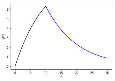
Exercise: Solve $\frac{dn}{dt} = -\lambda n + s(t)$ where

\[\begin{split}s = \left \{ \begin{array}{cc} 10^{6} & t \leq 10 \\ 0 & t > 10 \end{array} \right . \, ,\end{split}\]

$\lambda = 10^{-3}$, and $y(0) = 0$. Plot your result for $t \in [0, 30]$.

Solution: This problem is a bit tricky because the forcing function $s(t)$ is discontinuous. Here’s one way to tackle this. First solve for $0 \leq t \leq 10$. This part is identical to the last exercise. Then, with that solution, $y(10)$ is known, and this can be used as the initial value for $t > 10$. This part is identical the in-text example $y'=ay$.

In [9]:

# Define all the symbols needed.  However, be
# careful with "lambda"!  Remember, it's a keyword
# in Python.  Here, add an underscore.
y, y_0, t, lambda_, s, C1 = sy.symbols('y y_0 t lambda s C1')

# Devine the IVP in the first region and solve like
# the last exercise:
#   1. define the ivp for t in [0, 10]
ivp1 = sy.Eq(sy.diff(y(t), t), -lambda_*y(t) + s)
#   2. solve the ivp
sol1 = sy.dsolve(ivp1)
#   3. solve for the constant of integration by applying
#      the initial condition
ic = sy.Eq(sol1.rhs.subs(t, 0), y_0)
C = sy.solve(ic, C1)[0]
#   4. subsitute the constant along with s and lambda
y_sol1 = sol1.rhs.subs({C1: C, y_0: 0, s: 1, lambda_: 10**-1}).simplify()
y_sol1

Out[9]:

\[$$10.0 - 10.0 e^{- 0.1 t}$$\]

In [10]:

# Now, define the IVP in the second region.  We cannot use
# the original ivp1 because the two IVPs are different.  One
# has s and one does not.
#   1. define the ivp for t in [10, oo]
ivp2 = sy.Eq(sy.diff(y(t), t), -lambda_*y(t))
#   2. solve this ivp
sol2 = sy.dsolve(ivp2)
#   3. define the initial value y(10) using previous solution
y_10 = y_sol1.subs(t, 10)
#   4. solve for the constant of integration
ic = sy.Eq(sol2.rhs.subs(t, 10), y_10)
C = sy.solve(ic, C1)[0]
#   5. substitute this constant and others into the final result
y_sol2 = sol2.rhs.subs({C1: C, lambda_: 10**-1}).simplify()
y_sol2

Out[10]:

\[$$17.1828182845905 e^{- 0.1 t}$$\]

In [11]:

# Now, plot
import matplotlib.pyplot as plt
import numpy as np
t_plot1 = np.linspace(0, 10)
y_plot1 = sy.lambdify(t, y_sol1)(t_plot1)
t_plot2 = np.linspace(10, 30)
y_plot2 = sy.lambdify(t, y_sol2)(t_plot2)
plt.plot(t_plot1, y_plot1, 'k', t_plot2, y_plot2, 'b')
plt.xlabel('t')
plt.ylabel('y(t)')
plt.show()

../_images/lectures_ME400_Lecture_26_22_0.png

Exercise: My kid hates hot food, so if I make him my (absolute delicious grilled-cheese sandwich with 100% real Wisconsin cheese [of course]), I’ve got to let it cool down to approximately room temperature (say 70 ${}^{\circ}$F). If immediately after grilling it, the sandwich is 150 ${}^{\circ}$F, and 5 minutes later, it is 100${}^{\circ}$, how much longer do I have to let it cool? Assume that Newton’s law of cooling, $T' = k(T-T_m)$, applies. (Hint: you do have enough information to solve this problem.)

Exercise: Radio-carbon dating is a technique used to determine how old fossils are. The technique is based on the fact that the radioactive isotope C-14 is produced in the atmosphere at an approximately constant rate. Living, breathing creatures have C-14 at levels consistent with the atomosphere. Dead, fossilized creatures have C-14 levels that decrease over time. The half life of C-14 is about 5600 years, meaning that every 5600 years, the amount of C-14 in the fossil will decrease by half. Use this number and the simple model $N' = -\lambda N(t)$ (where $N$ represents the amount of C-14) to determine $\lambda$. Then, determine how old a fossil must be if its C-14 concentration is only 1/100 of that of a living creature.

Exercise: Try solving the nonlinear logistics equation: $y' = y(t)[a - by(t)]$ with $y(0) = y_0$. Can SymPy do this? This model extends the exponential growth model $y'/y = a$ by $y'/y = a - by$. The $-by$ term represents some sort of inhibitor for unbounded growth. Think about it: unbounded growth would require unbounded resources. In the real world, those resources are not available, and so there tends to be muted growth as populations become very large. This reduction in the grown rate can be modeled as being proportional to the population itself, leading to this nonlinear model. Plot the solution for $y(0) = 1$, $a = 1$, and $b = 0$ and $b = 1$. Notice a difference?

Second-Order Problems¶

Many models in engineering involve high-order derivatives. Here, we’ll focus only on second-order differential equations.

Second-Order IVPs¶

A good first application is the spring-mass system. Specifically, consider the equation

\[m \frac{d^2 x}{dt^2} = -k x - a \frac{dx}{dt} \, ,\]

which represents Newton’s second law for a spring-mass system with spring constant $k$ and damping force $a$. Here, we’ll be solving this equation subject to the ICs $x(0) = x_0$ and $x'(0) = v_0$.

Exercise: If $x$ is in units of m and $m$ is the mass in kg, what are the units for $k$ and $a$?

Exercise: Solve the spring-mass equation above for $x(0) = x_0$ and $x'(0) = v_0$.

In [12]:

# Define all symbols
x, x_0, v_0, t, m, k, a = sy.symbols('x, x_0, v_0, t, m, k, a')

In [13]:

# Define the IVP
ivp = sy.Eq(m*sy.diff(x(t), t, 2), -k*x(t) - a*sy.diff(x(t), t))
ivp

Out[13]:

\[$$m \frac{d^{2}}{d t^{2}} x{\left (t \right )} = - a \frac{d}{d t} x{\left (t \right )} - k x{\left (t \right )}$$\]

In [14]:

# Solve the IVP
sol = sy.dsolve(ivp)
sol

Out[14]:

\[$$x{\left (t \right )} = C_{1} e^{\frac{t}{2 m} \left(- a - \sqrt{a^{2} - 4 k m}\right)} + C_{2} e^{\frac{t}{2 m} \left(- a + \sqrt{a^{2} - 4 k m}\right)}$$\]

In [15]:

# Define the ICs
ic1 = sy.Eq(sol.rhs.subs(t, 0), x_0)
ic2 = sy.Eq(sy.diff(sol.rhs, t, 1).subs(t, 0), v_0)
ic1, ic2

Out[15]:

\[$$\left ( C_{1} + C_{2} = x_{0}, \quad \frac{C_{1}}{2 m} \left(- a - \sqrt{a^{2} - 4 k m}\right) + \frac{C_{2}}{2 m} \left(- a + \sqrt{a^{2} - 4 k m}\right) = v_{0}\right )$$\]

In [16]:

# Solve for the undetermined coefficients
coefs = sy.solve([ic1, ic2], [sy.Symbol('C1'), sy.Symbol('C2')])
coefs # remember, it's a dictionary now

Out[16]:

\[$$\left \{ C_{1} : \frac{1}{\sqrt{a^{2} - 4 k m}} \left(- \frac{a x_{0}}{2} - m v_{0} + \frac{x_{0}}{2} \sqrt{a^{2} - 4 k m}\right), \quad C_{2} : \frac{1}{\sqrt{a^{2} - 4 k m}} \left(m v_{0} + \frac{x_{0}}{2} \left(a + \sqrt{a^{2} - 4 k m}\right)\right)\right \}$$\]

In [17]:

# Substitute these coefficients back into the solution
sol_x = sol.rhs.subs(coefs).simplify()
sol_x

Out[17]:

\[$$\frac{e^{- \frac{a t}{m}}}{2 \sqrt{a^{2} - 4 k m}} \left(\left(2 m v_{0} + x_{0} \left(a + \sqrt{a^{2} - 4 k m}\right)\right) e^{\frac{t}{2 m} \left(a + \sqrt{a^{2} - 4 k m}\right)} + \left(- a x_{0} - 2 m v_{0} + x_{0} \sqrt{a^{2} - 4 k m}\right) e^{\frac{t}{2 m} \left(a - \sqrt{a^{2} - 4 k m}\right)}\right)$$\]

Exercise: Let $m = 1$ and $k = 1$ in the solution for the spring-mass system above. Plot the solution for $a = 1$, $a=2$, and $a=3$ over the times $t\in [0, 10]$ assuming $x_0 = 1$ and $v_0 = 1$.

Second-Order BVPs¶

Boundary-value problems (BVPs) are of critcal importance for many physical models, including those of heat conduction through media and neutron diffusion in nuclear reactors. We’ll stick with second-order equations with constant coefficients, i.e., equations of the form

\[\frac{d^2 y}{dx^2} + p\frac{dy}{dx} + q y(x) = s(x) \, ,\]

where $s(x)$ is an arbitrary forcing function. Boundary conditions specify $y(x)$ or its derivative at two separate points $x = a$ and $x = b$. That makes the equation a two-point BVP.

Recall, the equation is homogeneous if $s(x) = 0$, and inhomogenous otherwise. The general solution to such equations is the sum of the homogeneous solution (i.e., the solution when $s(x) = 0$) and the particular solution. There are a variety of tricks for solving such equations, but that’s not our focus; rather, we’ll leverage SymPy for the general solution and apply boundary conditions (BCs) to develop final solutions.

More specifically, here’s our approach, and it follows what we’ve done for IVPs: 1. Define the BVP 2. Solve the BVP using dsolve 3. Define the BCs 4. Solve the BCs to define the two undetermined constants 5. Substitute those constants (and any other values) to the general solution 6. Perform any plotting, etc., required by the problem statement.

Exercise: Solve the heat equation $k\frac{d^2 T}{dx^2} = 0$ subject to $T(0) = 0$ and $T(a) = 100$. By the way, this equation models the temperature $T$ through a wall of thickness $a$ whose left and and right surfaces are held at 0 and 100 K, respectively.

Solution

In [18]:

# 1. Define the BVP
T, x, k, a = sy.symbols('T, x, k, a')
bvp = sy.Eq(k*sy.diff(T(x), x, 2), 0)
bvp

Out[18]:

\[$$k \frac{d^{2}}{d x^{2}} T{\left (x \right )} = 0$$\]

In [19]:

# 2. Solve the BVP using dsolve
sol = sy.dsolve(bvp)
sol

Out[19]:

\[$$T{\left (x \right )} = C_{1} + C_{2} x$$\]

In [20]:

# 3. Define the BCs
bc_left = sy.Eq(sol.rhs.subs(x, 0), 0)
bc_right = sy.Eq(sol.rhs.subs(x, a), 100)
bc_left, bc_right

Out[20]:

\[$$\left ( C_{1} = 0, \quad C_{1} + C_{2} a = 100\right )$$\]

In [21]:

# 4. Solve the BCs for C1 and C2
coefs = sy.solve([bc_left, bc_right], sy.symbols('C1'), sy.symbols('C2'))
coefs

Out[21]:

\[$$\left \{ C_{1} : 0, \quad C_{2} : \frac{100}{a}\right \}$$\]

In [22]:

# 5. Substitutions
sol_T = sol.rhs.subs(coefs)
sol_T

Out[22]:

\[$$\frac{100 x}{a}$$\]

The temperature found is linear, and it varies from 0 (at the left) to 100 (at the right). Does the solution depend on the conductivity $k$? (Remember, $k$ quantifies how readily heat transfers through a medium by conduction.)

Exercise: Solve the heat equation $k\frac{d^2 T}{dx^2} = 1$ subject to $T(0) = 0$ and $T(a) = 100$. What happens to $T$ within the wall as $k$ is increased?

Exercise: Solve the heat equation $k\frac{d^2 T}{dx^2} = 1$ subject to $T(0) = 0$ and $T'(a) = 0$. The condition $T'(a)$ is we specify the right surface of the wall to be perfectly insulating. If $T'$ vanishes, so does the heat flux $kT'$, and if not heat is passing through, we’re insulated.

Exercise: Consider the second-order, ordinary differential equation

\[-D \frac{d^2 \phi}{dx^2} + \Sigma \phi(x) = S(x) \, ,\]

which is one (albeit simplified) model for the diffusion of neutron particles in a 1-D system. Two possible applications of this model include (1) the transport of energy via radiation (i.e., radiation heat transfer) and (2) the diffusion of neutrons in a nuclear reactor.

Consider the case for which $\phi(0) = \phi(10) = 0$, $D = 1/3$, $\Sigma = 1/2$, and

\[\begin{split}s = \left \{ \begin{array}{cc} 1 & x \leq 5 \\ 0 & 0 > 5 \end{array} \right . \, .\end{split}\]

To solve this problem, assume that $\phi(x)$ and $D \frac{d \phi}{dx}$ must be continuous at $x = 5$. For heat transfer, this continuity means the temperature and the heat flux are continuous. For neutron diffusion, this means the neutron flux and its current are continuous. (Hint: Solve the equation separately for $x \leq 5$ and $x > 5$. Then, the BCs and the continuity conditions provide 4 equations for the four undetermined coefficients.)

Exercise: Consider the following partial differential equation (PDE):

\[\frac{\partial c}{\partial t} = D(x) \frac{\partial^2 c}{\partial x^2} - v(x)\frac{\partial c}{\partial x} + S(x)\]

which is a simplified, one-dimensional, advection-diffusion equation. Here, $c(x)$ is the concentration of some quantity of interest (perhaps a pollutant in a stream), $D$ is a diffusion coefficient (that quantifies how rapidly the species tends to dissipate away from a region in space), and $v(x)$ is the velocity of the surrounding field (here, perhaps the stream with the pollutant).

Like many equations that model physical systems, the convection-diffusion equation is a statement of balance. On the left, we have $\frac{\partial c}{\partial t}$, which is the time rate of change of the concentration at any point $x$. This change comes from three sources:

the diffusion of the species away from a point $x$, here quantified by $D(x) \frac{\partial^2 c}{\partial x^2}$
the advection of the species away from a point $x$ due to the flow of the surrounding field (here, again, the stream), here quantified by $-v(x)\frac{\partial c}{\partial x}$
any external sources of the species, perhaps a leaking canister or a chemical reaction, here represented by $S(x)$

Now, do the following:

Suppose the unit of $c$ is m$^{-3}$. What must be the units of $D$, $v$, and $S$?
Write down the steady-state form of the above convection-diffusion equation by setting the time derivative to zeros.
Solve the steady-state equation for the case $v = 1$, $S = 1$, $c(0) = 0$ and $c(10) = 1$.
Plot your solution for $D = 10$, $D = 1$, and $D = 0.1$. What happens? (The phenomenon you should observe is the development of a boundary layer, a term that should become familiar in fluid mechanics.)