Lecture 27 - Solving First-Order IVPs Numerically
Overview, Objectives, and Key Terms
The basics of ODEs were reviewed in Lecture
26. There, SymPy was used to provide general
solutions via dsolve, leaving application of initial and boundary
conditions to the user. However, SymPy (and other symbolic tools) cannot
solve all differential equations. For such equations, we can apply
numerical techniques. Specifically, we’ll apply the finite-difference
approximations presented in Lecture 19. For
now, we’ll consider only single, first-order equations, leaving systems
for Lecture 28.
Objectives
By the end of this lesson, you should be able to
- Solve first-order IVPs numerically using forward and backward Euler’s method
- Explain what is mean by local and global errors
- Explain what is meant by stability and how to achieve it
Prerequisites
You should already be able to
- Solve ODEs based on what you’ve learned in a course like MATH 340 and Lecture 26
- Compute a first-order, finite-difference approximation for \(\frac{df}{dx}\)
Key Terms
- Euler’s method
- forward Euler
- backward Euler
- Heun’s (improved Euler’s) method
- local error
- global error
- stable method
scipy.integrate.odeint
There Once was a Man Named Euler
Leonhard Euler was a prolific mathematician, perhaps second only to Carl Gauss. I point him out because the simplest (and probably best known) approach for solving \(y' + py = q\) has his name. (Point of trivia: he’s buried in St. Petersburg, I was quite surprised to learn while strolling through an old cemetery).
The method bearing his name requires the Numerical Differentiation we learned previously. Specifically, we need one of the first-order, finite-difference approximations for \(dy/dt\). You’ll recall those are the forward difference
and the backward difference
If we substitute the forward difference into the IVP, we find
and by collecting the terms with \(y(t)\) on the left, we have
Recognize that \(y\) is now evaluated at the points \(t_0, t_0+\Delta, t_0+2\Delta, \ldots\), or
We could allow for a \(\Delta\) that changes, but we’ll keep it fixed for simplicity and leave the fancy stuff to SciPy. Furthermore, let \(y(t_{n})\) be written as \(y_n\). Then, we can rewrite our finite-difference equation as
which is the forward Euler method. Use of the backward difference leads to the backward Euler method
which is a stable time-integration scheme for IVP’s. For both methods, the \(\mathcal{O}(\Delta^2)\) error in the derivative leads to a a local error of \(\mathcal{O}(\Delta)\) in the solution.
How high should \(n\) go? It depends on how long into the future (taking \(t\) to represent time) we wish to evaluate the solution. Let that future time be denoted \(T\), and let the number of steps we wish to take be denoted \(N\). Consequently, \(\Delta = (T-t_0)/N\). We’ll always start at \(t=0\), so \(\Delta = T/N\).
Let’s illustrate by solving
using \(N=25\) points.
In [1]:
import numpy as np
%matplotlib inline
import matplotlib.pyplot as plt

t_max = 10.0
N = 25

# Initialize the unknown (where "fe25" denotes Forward Euler with 15 points)
y_fe25 = np.zeros(N+1)

# Define the times and right-hand side.  We use N+1
# because we want N points beyond the initial value.
t_fe25 = np.linspace(0, t_max, N+1)
q = 10*np.ones(N+1)
Delta = t_fe25[1]-t_fe25[0]

# Compute all successive values
for i in range(1, N+1) :
    y_fe25[i] = (1.0 - Delta)*y_fe25[i-1] + Delta*q[i-1]

plt.plot(t_fe25, y_fe25, 'k-o')
plt.xlabel('t')
plt.ylabel('$y(t)$')
plt.show()
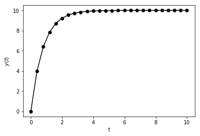
Is this reasonable? You should always do any “sanity” check available. Here, the solution looks like it levels off, which suggests for long times, a steady state is reached. Steady state means no change with time, and no change with time means \(dy/dt = 0\).
So what happens if we set \(dy/dt=0\) in our IVP? We find that \(y(t) = 10\). That seems consistent with the numerical result, but is it correct? This problem is easy to solve directly, but we’ll have SymPy produce an analytic result that be evaluated numerically later on:
In [2]:
import sympy as sy
sy.init_printing()
y_sy, t_sy = sy.symbols('y t') # use y_sy, t_sy to avoid overwriting other names
sol = sy.dsolve(sy.diff(y_sy(t_sy), t_sy) + y_sy(t_sy)-10, y_sy(t_sy)).rhs
y_exact_sy = sol.subs(sy.Symbol('C1'), sy.solve(sol.subs(t_sy, 0), sy.Symbol('C1'))[0])
y_exact_sy
Out[2]:
That certainly goes to 10 as \(t \to \infty\). Let’s visualize the numerical and analytical solutions:
In [3]:
y_exact = sy.lambdify(t_sy, y_exact_sy)
plt.plot(t_fe25, y_fe25, 'k-o', t_fe25, y_exact(t_fe25), 'r--')
plt.xlabel('t')
plt.legend(['$y_{\\mathrm{fe25}}$', '$y_{\\mathrm{exact}}(t)$'], loc=0)
plt.show()
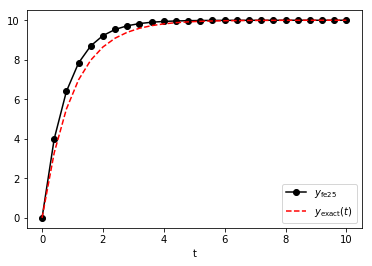
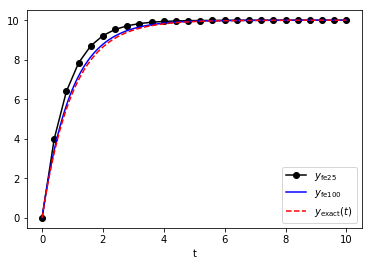
That’s pretty close, but can we do better? Let’s try \(N=100\):
In [4]:
N = 100

# Initialize the unknown (where "fe25" denotes Forward Euler with 15 points)
y_fe100 = np.zeros(N+1)

# Define the times and right-hand side.  We use N+1
# because we want N points beyond the initial value.
t_fe100 = np.linspace(0, t_max, N+1)
q = 10*np.ones(N+1)
Delta = t_fe100[1]-t_fe100[0]

# Compute all successive values
for i in range(1, N+1) :
    y_fe100[i] = (1.0 - Delta)*y_fe100[i-1] + Delta*q[i-1]

plt.plot(t_fe25, y_fe25, 'k-o', t_fe100, y_fe100, 'b', t_fe100, y_exact(t_fe100), 'r--')
plt.xlabel('t')
plt.legend(['$y_{\\mathrm{fe25}}$', '$y_{\\mathrm{fe100}}$', '$y_{\\mathrm{exact}}(t)$'], loc=0)
plt.show()
Exercise: Finish the following function definition:
def forward_euler(N, T, y0, p, q) :
    """Solves y' + py = q using forward Euler and a fixed time step.

       Inputs:
         N  - number of points (int)
         T  - final time (float)
         y0 - initial value of y (float)
         p  - coefficient value (float)
         q  - coefficient value (float)

       Returns:
         y  - values of y at each time step (NumPy array)
         t  - times at which y is evaluated (NumPy array)
    """

    return y, t
Exercise: Repeat the last exercise but allow p and q to be
callable functions of t.
Exercise: Implement backward Euler following the exercise above.
Exercise: Apply forward Euler by hand to the following IVPs to approximate \(y(1)\) using a step size \(\Delta = 0.2\): 1. \(y' = y\) for \(y(0) = 1\). 2. \(y' = 2ty\) for \(y(0) = 1\) 3. \(y' = -y/10 + 1\) for \(y(0) = 0\).
Exercise: Repeat the previous exercise but use backward Euler.
Exercise: Consider \(y' = y\), \(y(0) = 1\). Of course, the solution is \(y(x) = e^x\). Let \(\Delta = 1/N\) and \(x_i = \Delta i\), where \(N\) is some integer. If \(y_i\) is the approximation of \(y(x)\) at \(x = x_i\), then prove that \(\lim_{N\to \infty} y_N = e\) for both forward Euler and backward Euler.
Exercise: Consider the IVP \(y' = f(t, y(t))\) subject to \(y(0) = y_0\). Here, \(f(t, y(t))\) can be any function of \(t\) or \(y(t)\). Examples include \(f(t, y(t)) = ay + bt\) and \(f(t, y(t)) = a y(t)^2\). The latter case leads to a nonlinear IVP. Given the initial condition, write down how you would determine \(y(\Delta)\) using (a) forward Euler and (b) backward Euler.
Exercise: Consider the following twist on Euler’s method for \(\frac{dy}{dt} = f(t)\) using fixed time steps \(\Delta\):
and
This is an example of a multi-step method and belongs to the famous Runge-Kutta family of methods. This particular version is sometimes called Heun’s method.
Your task is to write a function heun_method(N, T, y0, p, q).
A Look at Errors and Stability
Certainly, the \(N=100\) approximation looks better than the \(N=25\) approximation. We can plot the errors for both as a function of time:
In [5]:
error_fe25 = y_fe25 - y_exact(t_fe25)
error_fe100 = y_fe100 - y_exact(t_fe100)
plt.semilogy(t_fe25, error_fe25, 'k-', t_fe100, error_fe100, 'b--')
plt.xlabel('t')
plt.legend(['$N=25$', '$N=100$'], loc=0, numpoints=1)
plt.show()
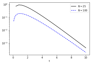
Clearly, the error for \(N=25\) is larger over the time domain, as we might expect. Recall that \((y_{n+1}-y_n)/\Delta = -py_n + q_n + \mathcal{O}(\Delta^2)\), so \(y_{n+1} = (1-\Delta p)y_n + \Delta q_n + \mathcal{O}(\Delta)\). This first-order error in \(y_n\) is the local error, i.e., the error introduced by a single step in time. On the other hand, the global error is the error shown above as a function of time. A key question is how that global error at a fixed point in time depends on \(\Delta\). It turns out that if a method is stable, then the global error is of the same order as the local error.
We’ll skip momentarily what it means to be stable for now, but we can attack the global error for our simple problem (with a bit of help from SymPy). For constant \(q\), \(p\) and \(\Delta\), the analytic solution is
while the forward-Euler solution is
For fixed \(t\) and \(\Delta\), the number of steps is \(n = t/\Delta\), and the global error is therefore
Note first that
so \(e_n = (q/p)[e^{-pt}-e^{-p/t}/(1-\Delta p)] \to 0\) as \(\Delta \to 0\). However, for fixed \(t\), how fast does that error decrease with \(\Delta\)? And for fixed \(\Delta\), how does the error change with time? Let’s expand the error about \(\Delta = 0\):
In [6]:
y0, Delta, n, p = sy.symbols('y0 Delta n p')
e = y0*(sy.exp(-p*t_sy)-(1-Delta*p)**(t_sy/Delta-1))
sy.series(e, Delta, 0, 3)
Out[6]:
Evidently, the global error is of first order, consistent with the local error. However, it’s not clear (or easy to determine) exactly how the error depends on \(t\) for fixed \(\Delta\). If we assume \(p > 0\) (i.e., radioactive decay and not multiplying pythons), then
However, the right-hand side is bounded (i.e., does not grow with large \(t\)) only if \(|1-\Delta p| < 1\), and that is true only if \(\Delta < 2/p\). To summarize: the global error does not blow up as long as \(p > 0\) and \(\Delta < 2/p\).
Of course, simply stating such rules is never as exciting as seeing what happens when the rules are broken, so we’ll solve our example with \(p = 2\), \(q=10\), and \(y(0) = 0\) for \(N = 5\), \(N = 10\), and \(N = 20\):
In [7]:
p = 2.0
q = 10.0
t = {}
y = {}
y0 = 0
for N in [5, 10, 20]:
    t[N] = np.linspace(0, 10, N+1)
    Delta = t[N][1]-t[N][0]
    y[N] = np.zeros(N+1)
    y[0] = y0
    for i in range(1, N+1):
        y[N][i] = (1.0 - Delta*p)*y[N][i-1] + Delta*q

plt.plot(t[5], y[5], 'k-o', t[10], y[10], 'b-s', t[20], y[20], 'r-*')
plt.xlabel('t')
plt.ylabel('y(t)')
plt.legend(['$N=5$', '$N=10$',  '$N=20$'], loc=0)
plt.show()
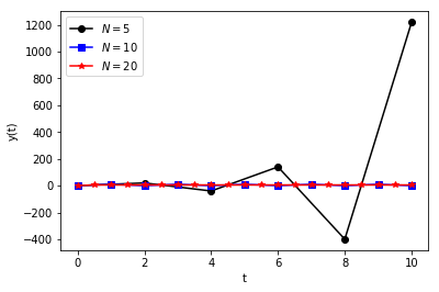
Yikes! The \(N=5\) case clearly does not converge to the steady-state value \(y = 5\)! In other words, it diverges. Because the forward-Euler approximation converges only for certain values of \(\Delta\) and \(p\), it is called a conditionally stable method.
Conditional stability requires very small \(\Delta\). For problems whose solutions blow up (i.e., \(p < 0\)), all bets are off and an unconditionally stable method is the better choice. For example, the backward-Euler approximation is unconditionally stable, demonstration of which is an exercise left to the student.
Exercise: Repeat the example above (i.e., \(p=2\), \(q=10\), \(y(0) = 0\), and \(N = 5, 10, 20\)) to show that backward Euler has no stability issues.
Exercise: Use backward Euler to solve \(y' = 2t - 3y + 1\) given \(y(1) = 5\) and estimate \(y(1.2)\). Compare the error in this estimate for \(\Delta = 0.1, 0.01, 0.001, 0.0001\). How does this error depend on \(\Delta\)?
Exercise: Repeat the previous exercise using Heun’s method (see previous exercise).
IVP’s with SciPy
SciPy includes a number of schemes for integration (e.g., the
scipy.integrate.quad function we have previously used). The
scipy.integrate module also has routines for integrating IVP’s. To
“integrate” a differential equation is to solve for the unknown
function.
Specifically, the scipy.integrate.odeint function is used to solve
individual, first-order IVP’s or systems of such equations. We’ll focus
only on the former, leaving systems for next time. Behind the scenes,
either an
Adams
or
BDF
method is used depending on the behavior of the solution. All of this is
automatic, and more details can be found in the
documentation.
Let’s revisit our example, namely \(y' + y(t) = 10\) with
\(y(0)=0\) for \(t\in [0, 10]\). The odeint function
requires, at a minimum, three inputs: (1) a function that evaluates the
derivative \(y'(t)\) given the time \(t\) and the value of the
function \(f(t)\), (2) the initial condition \(y(0)=y_0\), and
(3) the times at which \(y(t)\) is to be evaluated. These times are
independent of the times and corresponding \(\Delta\)‘s used
internally; they only are used for the output.
The derivative function has two arguments: the time \(t\) at which
\(y'\) is to be evaluated, and the value of \(y\) at that same
time. That sounds like you need to know \(y(t)\) beforehand—but
you don’t! This derivative function is only called behind the scenes by
odeint itself. Hence, odeint knows (or has an approximation to)
\(y\) at the time \(t\), and your job is to use the two to
define \(y'\). For our example, that means we need a function that
evaluates and returns
With that, we can implement a complete odeint solution to our
example:
In [8]:
from scipy.integrate import odeint

# derivative function
def y_prime(y, t) :
    return 10.0 - y

# times at which y(t) is to be evaluated
t_odeint = np.linspace(0, 10)

# solve with odeint
y_odeint = odeint(y_prime, y0=0.0, t=t_odeint)

plt.plot(t_odeint, y_odeint, 'k', t_odeint, y_exact(t_odeint), 'ro')
plt.legend(['$y_{\\mathrm{odeint}}$', '$y_{\\mathrm{exact}}$'], loc=0, numpoints = 1)
plt.show()
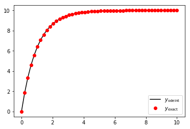
The odeint result is very good, with no discernible error (to my
eyes, anyway). We can plot the errors, but first we need to reshape the
output from odeint. Notice that it has an explicit, 2-D shape,
whereas y_exact yields a 1-D array (from the 1-D t_odeint):
In [9]:
print(y_odeint.shape)
print(y_exact(t_odeint).shape)
print(t_odeint.shape)
(50, 1)
(50,)
(50,)
Normally, this apparent mismatch is no big deal—we plotted both
against the same t_odeint array. However, the mismatch does lead to
strange results when we try to compute the error:
In [10]:
error = y_odeint-y_exact(t_odeint)
print(error.shape)
(50, 50)
That’s not right—can you figure out why that is happening? The solution, however, is to make them the same size, and we can do that, e.g., with an explicit reshaping:
In [11]:
y_odeint_reshaped = y_odeint.reshape((len(t_odeint),))
error = y_odeint_reshaped - y_exact(t_odeint)
print(error.shape)
(50,)
In [12]:
plt.plot(t_odeint, error, 'r-o')
plt.xlabel('t')
plt.ylabel('$y_{\\mathrm{odeint}}-y_{\\mathrm{exact}}$')
plt.show()
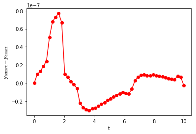
Two features of this error warrant discussion. First, the overall
magnitude is small than the errors we found using \(N=100\) above
with forward Euler. Second, the error fluctuates more than we found for
forward Euler and is more uniform in magnitude. The overall magnitude of
the error is determined by the desired numerical accuracy (defined by
the optional arguments rtol and atol). The time-dependent
fluctuations are due to use of nonuniform time steps. The details are
well beyond our scope, but you’ll recall from the Taylor expansion of
\(y'\) that the errors are related to \(y''\). If some estimate
can be made of \(y''\) during the time-stepping procedure, then the
error can also be estimated. Proper selection of \(\Delta\) (either
larger or smaller) can yield errors just within the desired tolerance,
ensuring proper accuracy and avoiding use of too many small steps in
regions where they are not needed.
Exercise: Solve the following IVPs using odeint and plot the
result for \(t \in [0, 5]\):
- \(\frac{dy}{dt} = e^{-y}\) for \(y(0) = 0\).
- \(\frac{dy}{dt} = x^2 + y^2\) for \(y(0) = 1\).
- \(\frac{dy}{dt} = y - y^2\) for \(y(0) = 0.5\).
Further Reading
See the SciPy documentation on odeint. This will also be useful for the next lesson in which systems of IVP’s (and higher-order IVP’s) are solved. Bennett’s chapter on population growth provides a bit more on first-order systems and their use in modeling populations.