Numerical Solutions of Two-Point BVPs

Overview, Objectives, and Key Terms

This lesson is all about solving two-point boundary-value problems numerically. We’ll apply finite-difference approximations to convert BVPs into matrix systems. Both inhomogeneous cases (e.g., heat conduction with a driving source) and homogeneous (a critical nuclear reactor) will be considered.

Objectives

By the end of this lesson, you should be able to

• Solve two-point, heterogeneous BVPs.
• Solve two-point, homogeneous BVPs.

Prerequisites

You should already be able to

• Solve systems of IVPs using Euler’s method
• Define one- and two-dimensional arrays using NumPy arrays
• Use np.linalg.solve to solve \(\mathbf{Ax = b}\)

Please review these topics (and resources) as needed.

Key Terms

• Dirichlet boundary condition
• Neumann boundary condition
• Robin (or mixed) boundary condition

Chopping Up the BVP

Our focus is again on the second-order BVP

\[\frac{d^2 y}{dx^2} + p(x) \frac{dy}{dx} + q(x) y(x) = f(x), \qquad y(a) = y_a, \qquad y(b) = y_b \, .\]

The goal is to apply numerical differentiation to this equation, leading to a linear system.

Observe that there are two derivatives in the BVP, one second order, and one first order. There are numerous ways to approximate these by finite differences, but we’ll opt for a method with second-order errors. For the first derivative, we already analyzed the central difference:

\[\frac{dy}{dx} = \frac{y(x+\Delta)-y(x-\Delta)}{2\Delta} + \mathcal{O}(\Delta^2) \, .\]

For the second derivative, we saw (but did not analyze) another central difference:

\[\frac{d^2y}{dx^2} = \frac{y(x+\Delta)-2y(x)+y(x-h)}{\Delta^2} + \mathcal{O}(\Delta^2) \, .\]

Given these differencing schemes, let us chop the domain \(x\in [a, b]\) into discrete points \(x_i = a + \Delta i,\, i = 0, 1, \ldots, n\), where \(\Delta = (b-a)/n\). For all but \(i=0\) and \(i=n\), we have

\[\frac{y_{i+1} - 2y_i + y_{i-1}}{\Delta^2} + p_i \frac{y_{i+1}-y_{i-1}}{2 \Delta} + q_i y_i = f_i\]

where, for example, \(y_i = y(x_i)\).

At the boundaries, we need to be more careful. For the given boundary conditions, our equations are as simple as

\[y_0 = y_a\]

and

\[y_n = y_b \, .\]

The boundary conditions used here are known as Dirichlet boundary conditions, in which the unknown function itself is defined at the boundary. Neumann boundary conditions specify a value of the derivative of the function, e.g., \(y'(a) = \alpha\). Robin or mixed boundary conditions specify a value of some linear combination of the function and its derivative, e.g., \(\gamma y'(a) + \beta y(a) = \alpha\). Dirichlet and Neumann conditions can be defined in terms of the Robin condition using appropriate values of \(\gamma\), \(\beta\), and \(\alpha\).

---

Exercise: Develop an equation to represent the Neumann condition \(y'(a) = \alpha\) based on finite differences. Here, \(x=a\) is the left boundary.

---

Exercise: Develop an equation to represent the Neumann condition \(y'(b) = \alpha\) based on finite differences. Here, \(x=b\) is the right boundary.

---

Exercise: Develop an equation to represent the Robin condition \(\gamma y'(a) + \beta y(a) = \alpha\) based on finite differences. Here, \(x=a\) is the left boundary.

Solution: Let \(y_0 = y(a)\) and \(y_1 = y(a+\Delta)\). Then approximate \(y'(a)\) as \([y_1 - y_0]/\Delta\) from which the boundary condition becomes

\[\frac{\gamma}{\Delta} y_1 + \left ( \beta - \frac{\gamma}{\Delta} \right ) y_0 = \alpha \, .\]

---

Exercise: Develop an equation to represent the Robin condition \(\gamma y'(b) + \beta y(b) = \alpha\) based on finite differences. Here, \(x=b\) is the right boundary.

---

A Simple Example

To illustrate the approach just described, let us consider our previous example for which \(p(x)=0\), \(q(x)=f(x)=-1\), and \(y(0) = y(10) = 0\). The analytic solution is \(y(x) = 1 - e^{10-x}/(1+e^{10}) - e^{x}/(1+e^{10})\). We’ll keep it simple and let \(n = 4\), which gives us five equations:

\[\begin{split}\begin{aligned} y_0 &= 0 \\ \frac{y_2 - 2y_1 + y_0}{\Delta^2} - y_1 &= -1 \\ \frac{y_3 - 2y_2 + y_1}{\Delta^2} - y_1 &= -1 \\ \frac{y_4 - 2y_3 + y_2}{\Delta^2} - y_1 &= -1 \\ y_4 &= 0 \end{aligned} \, .\end{split}\]

In matrix form, these become

\[\begin{split}\left [ \begin{matrix} 1 & 0 & 0 & 0 & 0 \\ 1/\Delta^2 & -2/\Delta^2 -1 & 1/\Delta^2 & 0 & 0 \\ 0 & 1/\Delta^2 & -2/\Delta^2 -1 & 1/\Delta^2 & 0 \\ 0 & 0 & 1/\Delta^2 & -2/\Delta^2 -1 & 1/\Delta^2 \\ 0 & 0 & 0 & 0 & 1 \\ \end{matrix} \right ] \left [ \begin{matrix} y_0 \\ y_1 \\ y_2 \\ y_3 \\ y_4 \\ \end{matrix} \right ] = \left [ \begin{matrix} 0 \\ -1 \\ -1 \\ -1 \\ 0 \\ \end{matrix} \right ] \, .\end{split}\]

In fact, we can simplify this system somewhat. Because we already know the values \(y_0\) and \(y_4\) from the boundary conditions, we can subsitute them into the equations for \(y_1\) and \(y_3\), which leads to

\[\begin{split}\left [ \begin{matrix} -2/\Delta^2 -1 & 1/\Delta^2 & 0 \\ 1/\Delta^2 & -2/\Delta^2 -1 & 1/\Delta^2 \\ 0 & 1/\Delta^2 & -2/\Delta^2 -1 \\ \end{matrix} \right ] \left [ \begin{matrix} y_1 \\ y_2 \\ y_3 \\ \end{matrix} \right ] = \left [ \begin{matrix} -1 \\ -1 \\ -1 \\ \end{matrix} \right ] \, .\end{split}\]

Personally, I like introducing the first version first since it puts all the equations together in a very transparent form. The second approach, however, leads to a somewhat simpler system. Note, though, this second approach is only applicable when the boundary condition is a Dirichlet condition.

Let’s solve this numerically:

import numpy as np
import matplotlib.pyplot as plt
Delta = 2.5
A = np.array([[1, 0, 0, 0, 0],
              [1/Delta**2, -2/Delta**2-1, 1/Delta**2, 0, 0],
              [0, 1/Delta**2, -2/Delta**2-1, 1/Delta**2, 0],
              [0, 0, 1/Delta**2, -2/Delta**2-1, 1/Delta**2],
              [0, 0, 0, 0, 1]])
b = np.array([0, -1, -1, -1, 0])
y_numerical = np.linalg.solve(A, b)
x = np.linspace(0, 10)
y_exact =  1.0 - np.exp(10-x)/(1+np.exp(10)) - np.exp(x)/(1+np.exp(10))
plt.plot(x, y_exact, 'k', [0, 2.5, 5.0, 7.5, 10], y_numerical, 'bo')
plt.legend(['exact', 'numerical'], loc=0, numpoints=1)
plt.show()

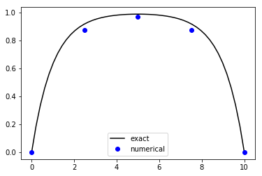
The approximation is not perfect, but then again, we used only five points!

---

Exercise: Apply the approach outlined above to solve \(y'' + y(x) = 1\), subject to \(y(0) = y(10) = 0\).

---

Exercise: Solve the convection-diffusion problem from Lecture 26 using finite differences.

---

Exercise: Apply the approach outlined above to solve \(y'' + y(x) = 1\), subject to \(y'(0) = y(10) = 0\). Note, that’s a Neumann condition at the left boundary.

---

Exercise: Use the finite-difference method to solve \(y'' + y(x) = x\), subject to \(y'(0) = y(10) = 0\).

---

Exercise: Implement the following function for solving arbitrary, second-order BVPs of the form \(y'' + p(x)y' + q(x)y(x) = s(x)\) subject to \(\gamma_a y(a) + \beta_a y'(a) = \alpha_a\) and \(\gamma_b y(b) + \beta_b y'(b) = \alpha_b\):

def bvp2(a, b, n, bc_a, bc_r, p, q, s):
    """ Solve y'' + p(x)y' + q(x)y(x) = s(x).

    Inputs:
        a - left boundary (float)
        b - right boundary (float)
        n - number of evenly spaced points (int)
        bc_a - tuple of three values
               (alpha, beta, gamma) for left condition
        bc_b - tuple of three values
               (alpha, beta, gamma) for right condition
        p - callable function for p(x)
        q - callable function for q(x)
        s - callable function for s(x)
    Returns:
        y - approximate function
        x - points at which y(x) is evaluated

---

Eigenvalue Problems

You may previously have studied the discrete, matrix eigenvalue problem:

\[\mathbf{Ax}=\lambda\mathbf{x} \, .\]

The eigenvalues \(\lambda\) are the roots of \(|\mathbf{A} - \lambda \mathbf{I}|\), where \(|\cdot|\) is the determinant. Here, that determinant leads to a polynomial equation for \(\lambda\). As long as \(\mathbf{A}\) is 4 by 4 or smaller, \(\lambda\) can be found directly. For larger matrices, we need numerical techniques (as was discussed in Lecture 23.

Eigenvalue problems are not limited to discrete systems, however. For example, consider the following BVP:

\[\begin{equation} - \frac{d^2 y}{dx^2} = \lambda y(x), \qquad y(0)=y(10)=0 \, . \end{equation}\]

This is really the homogeneous equation \(y'' - \lambda y = 0\), for which \(y(x) = a \cos(\sqrt{\lambda}x) + b \sin(\sqrt{\lambda}x)\). The left boundary condition \(y(0)=0\) gives \(a = 0\). However, the right condition leaves us with a somewhat strange situation:

\[\begin{equation} b \sin(\sqrt{\lambda}10) = 0 \, . \end{equation}\]

Why is this strange? All it says about \(b\) is that \(b=0\), the trivial solution. But if \(b\ne 0\), then it can be divided from both sides, leaving

\[\begin{equation} \sin(\sqrt{\lambda}10) = 0 \, . \end{equation}\]

Perhaps now our situation is a bit more obvious: the left boundary is not able to determine \(b\), but it is able to determine those values of \(\lambda\) for which the BVP and its boundary conditions are satisfied. Here, those values are

\[\begin{equation} \lambda = \frac{n^2 \pi^2}{100} \, . \end{equation}\]

Now, to solve such an equation, we can employ the same discretization used above, which leads to the following matrix eigenvalue problem:

\[\begin{equation} \left [ \begin{matrix} 1 & 0 & 0 & 0 & 0 \\ -1/\Delta^2 & 2/\Delta^2 & -1/\Delta^2 & 0 & 0 \\ 0 & -1/\Delta^2 & 2/\Delta^2 & -1/\Delta^2 & 0 \\ 0 & 0 & -1/\Delta^2 & 2/\Delta^2 & -1/\Delta^2 \\ 0 & 0 & 0 & 0 & 1 \\ \end{matrix} \right ] \left [ \begin{matrix} y_0 \\ y_1 \\ y_2 \\ y_3 \\ y_4 \\ \end{matrix} \right ] = \lambda \left [ \begin{matrix} y_0 \\ y_1 \\ y_2 \\ y_3 \\ y_4 \\ \end{matrix} \right ] \, . \end{equation}\]

We can solve this numerically via

A = np.array([[1, 0, 0, 0, 0],
               [-1/Delta**2, 2/Delta**2, -1/Delta**2, 0, 0],
               [0, -1/Delta**2, 2/Delta**2, -1/Delta**2, 0],
               [0, 0, -1/Delta**2, 2/Delta**2, -1/Delta**2],
               [0, 0, 0, 0, 1]])
l, v = np.linalg.eig(A)
print(l)

[ 0.54627417  0.32        0.09372583  1.          1.        ]

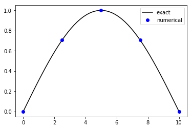
The smallest eigenvalue of the original equation comes with \(n=1\) (\(n=0\) is the trivial solution): \(\lambda_1 = \pi^2/100 \approx 0.0986960\), and the corresponding eigenfunction is \(y_1(x) = \sin(\pi x/10)\). Just as eigenvectors are defined only to within a multiplicative constant, so too are eigenfunctions.

The smallest eigenvalue found numerically is \(0.09372583\), which is pretty close to \(\pi^2/100\). Let’s look at the corresponding eigenvector compared to the analytic solution. We can make sure to pick out the correct eigenvector by finding the index of the lowest eigenvalue:

index_lowest = np.argmin(l)
print(index_lowest)

2

With that index, we can get the eigenvector and plot it with the analytic one (scaled so both have a maximum of one):

x = np.linspace(0, 10)
y_exact = np.sin(np.pi/10.*x)
y_numerical = v.T[index_lowest]
y_numerical = y_numerical/np.max(y_numerical)
plt.plot(x, y_exact, 'k', [0, 2.5, 5, 7.5, 10], y_numerical, 'bo')
plt.legend(['exact', 'numerical'], loc=0, numpoints=1)
plt.show()

For the other eigenvalues and eigenvectors, the numerical results are less impressive. For example, the next four eigenvalues are

for i in range(2, 6) :
    print(np.pi**2 * i**2 / 100)

0.3947841760435743
0.8882643960980423
1.5791367041742972
2.4674011002723395

and the list keeps going because \(n\) has no upper limit. The only way we can capture these higher modes is to have more points in our numerical solution. If the eigenvalues are viewed as frequencies, and the eigenfunctions as waves, it becomes obvious that too few points will prevent us from observing all the oscillations. However, usually our interest is in \(\lambda_1\) and \(y_1(x)\), for these correspond (in physical systems) to the fundamental or fundamental mode. That could be the critical spatial distribution of neutrons in a reactor, or the natural frequency of a cantileaver beam. Engineers (of one type of another) must analyze such systems, and numerical eigenvalues often play a role.

Comment on FDM and Alternatives

The finite-difference method is easy to understand, often simple to implement, and useful for a variety of real-world applications. However, it isn’t the only option and it’s often not the best option. Finite-volume methods (FVM’s) integrate the differential equation first, and the resulting \(\mathbf{Ax}=\mathbf{b}\) represents a discretetized conservation law. Finite-element methods (FEM’s) also integrate the differential equation first (albeit in a slightly different form). Then, the solutions are assumed to take simple piece-wise continuous form (lines, parabolas, or even cubics), and the integral balance over the whole domain becomes a linear system. Lots of details, but powerfully successful results.

These are two examples. Others include spectral methods, discontinuous-Galerkin methods, and boundary-element methods. There is a whole world to explore that goes well beyond the present scope (which, of course, is to solve problems).

Further Reading

Make sure to review the numerical differentiation and linear solver material previously covered.