Root Finding
Overview, Objectives, and Key Terms
In Lecture 19, SymPy was applied to perform symbolic differentuation, and in Lecture 21, finite-difference approximations were developed to perform numerical differentiation. We’ll need both techniques as we begin to solve nonlinear equations and optimization problems. Both subjects are rich, so we’ll touch on only the basics, but you’ll have tools at your disposal to tackle such problems in varied applications.
Objectives
By the end of this lesson, you should be able to
- Find one or more roots of a one-dimensional, nonlinear equation \(f(x) = 0\) using the bisection and Newton methods.
- Find local extrema of a function \(f(x)\) using the bisection and Newton methods.
- Use
fsolveto solve nonlinear systems. - Use
minimizeto solve nonlinear optimization problems.
Key Terms
- nonlinear equation
- transcendental equation
- graphical solution
- bisection method
- Newton’s method
- quadratic convergence
- second-order convergence
- order of convergence
- secant method
- Steffensen’s method
- nonlinear systems
- Jacobian matrix
scipy.optimize.fsolve- optimization
- extremum
- critical point
- objective function
scipy.optimize.minimize
Nonlinear Equations
Linear equations are characterized by linear combinations or the unknowns. For example, the system of equations for \(x\) and \(y\)
is linear because \(x\) and \(y\) appear with only constant coefficients. There are no \(x^2\) terms, or \(\sin(y)\) terms. Just multiples of \(x\) and \(y\). Any deviation from this pattern results in nonlinear equations. For example, quadratic equation \(ax^2 + bx + c = 0\) is nonlinear, and we know how to find the roots of this equations. A root is the solution \(x\) to any equation (generally, nonlinear) \(f(x) = 0\). Our goal now is to solve such equations using the tools at our disposal.
Analytic Solutions
In rare cases, nonlinear equations have closed-form solutions (i.e., you can write it down explicitly). The quadratic equation is one example. In fact, solutions exist for the general cubic (add a \(x^3\) term) and quartic (add both \(x^3\) and \(x^4\)). The roots are hideous (compared to the quadratic equation roots), but they are known.
Exercise: Use SymPy to find the roots of the cubic equation \(ax^3 + bx^2 + cx + d = 0\). Can it also find roots to quintic equation \(ax^5 + bx^4 + cx^3 + dx^2 + ex + f = 0\)?
Solution: The cubic is easy, but SymPy can’t do the quintic. In fact, the roots to general polynomials of degree 5 and higher cannot be determined explicity, a fact proven by Abel.
For other problems, we often have to have a bit of luck.
Exercise: Find all values of \(x\) such that \(\sin(ax) - b = 0\).
Solution: The equation has no solution if \(|b| > 1\) (because \(-1 \leq \sin(ax) \leq 1\)). If \(|b| \leq 1\), then \(x = \frac{\sin^{-1}b}{a} + n\pi\) for \(n = 0, \pm 1, \pm 2, \ldots\). Such an equation is called transcendental because it involves a transcendental function (i.e., \(\sin(x)\)). Transcendental functions cannot be defined in terms of polynomial of finite degree; in other words, if one needs an infinitely long Taylor series to represent the function, it is transcendental. Transcendental equations almost always require some form of numerical evaluation.
Exercise: Solve the nonlinear system of equations \(y - x = 4\) and \(x^2 + y = 3\).
Graphical Solutions
When analytic methods fail, solutions (albeit, approximate) to nonlinear equations may be found graphically. For single equation in \(x\), it suffices to plot \(f(x)\) over the range of interest and identify the roots.
Exercise: Revisit \(\sin(ax) - b\) for \(a=1\) and \(b=1/4\) and find all roots between \(x = -5\) and \(x = 5\).
Solution:
In [1]:
import matplotlib.pyplot as plt
import numpy as np
x = np.linspace(-5, 5, 100)
ax = plt.figure(1, (8,3)).gca()
plt.plot(x,  np.sin(x)-0.25, x, 0*x,'r--')
plt.xlabel('x')
plt.ylabel('f(x)')
ax.set_xticks(np.arange(-5, 6, 1))
plt.grid(True)
plt.show()
<Figure size 800x300 with 1 Axes>
Because plt.plot does not by default draw a line for \(y=0\), a
dashed, red line is superimposed to provide more obvious intersections
between the function \(f(x)\) and the horizontal axis \(y = 0\).
It appears (from inspections) that the roots of interest are near -3.5,
0.3, and 2.8. One could certainly zoom in somewhat to improve the
precision of the estimates, but arbitrary precision will require other
techniques.
Exercise: A simple, somewhat realistic model of a spherical nuclear reactor consists of two regions: (1) an inner spherical volume of fuel of radius \(R\), in which neutrons induce fission, leading to energy release and additional neutrons, and (2) an outer, infinitely large reflector surrounding the fuel, which minimizes the number of neutrons that escape the fuel. The reactor is critical if the number of neutrons produced and lost is constant over time. For this simple, two region model, the condition for criticality is
where \(D_f\), \(D_r\), and \(L_r\) are fixed, material properties of the fuel and reflector. Hence, in order for this criticality condition to be satisfied, an appropriate value of \(B\) must be determined. Here, \(B\) is called the buckling and is a function of several fuel material properties. For \(R=20\), \(D_f = 0.9\), \(D_r = 1.1\), and \(L_r = 1.7\), estimate the first positive value of \(B\) that satisfies the condition.
Exercise: The solution of transient heat-conduction problems often involves a technique called separation of variables. Application of this technique to an infinite slab of thickness \(2L\) subject to certain initial and boundary conditions leads to the transcendental equation
where \(\lambda\) is a dimensionless, undetermined parameter, \(h\) is the heat transfer coefficient, \(k\) is the thermal conductivity, and \(\text{Bi}\) is the Biot number. The Biot number quantifies how hard it is for heat to flow within a body relative to how hard it is to flow through the outer surface of the body. Only for certain values of \(\lambda\) can the equation be solved. Determine these values graphically by plotting the left-hand and right-hand sides of the equation as functions of \(\lambda L\).
Determining Roots Numerically
The numerical solution of \(f(x) = 0\) can be challenging since it requires we know at least a little about the desired solution, particularly the range in which the root is contained. We’ll explore three basic schemes for solving \(f(x)\): the bisection method, Newton’s method, and the secant method.
Bisection
Application of bisection to finding a root of \(f(x)\) requires a key piece of information: a range \(x \in [L, R]\) in which a single root lives. The algorithm is actually quite similar to binary search. A central point \(C\) is selected, and the function is evaluated at that point. Then, if \(f(C)\) has the same sign (i.e., \(+\) or \(-\)) as \(f(A)\), we know that the root must be between \(C\) and \(B\). Why? If there is only one root \(x^*\) between \(L\) and \(R\), then \(f(x)\) must have a constant sign for \(x \in [A, x^*)\) and the opposite sign for \(x \in (x^*, B]\). If, instead, \(f(x)\) changes signs between \(x=A\) and \(x=x^*\) then it must cross the \(x\) axis, at which point there must be a second root.
Exercise: Write a lambda function for \(x\) that returns
True if \(x \geq 0\) and False otherwise.
An important difference between bisection and binary search is that now the search can require an unlimited number of comparisons because the search range \([A, B]\) is split in half repeatedly until a root is converged to within a desired tolerance \(\tau\). In other words, roots will very rarely be found exactly; rather, we often must accept approximate values, as was first introduced earlier.
In pseudocode, the bisection method can be written as follows (where the notation from binary search is adopted as closely as is reasonable):
'''Bisection method for finding an isolated root of f between a and b'''
Input: f, a, b, tau

# Define the left and right boundaries
Set L = a
Set R = b

# Define the central point
Set C = (a+b)/2

# Go until f(C) is close enough to zero (i.e., that
# C is close enough to the root between a and b
While |f(C)| > tau
    If sign(f(C)) == sign(f(L)) then
        # the root must be between C and R
        L = C
    Otherwise
        # the root must be between L and C
        R = C
    C = (L+R)/2
Output: C
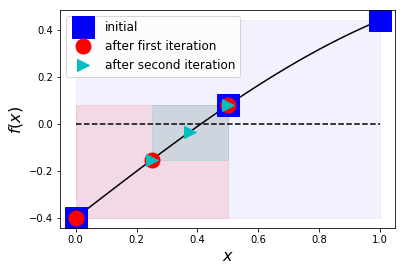
Application of this algorithm to find the first positive root of \(\sin(x) - 2/5\) is shown graphically below for the first two iterations. At each step, the search space is reduced by half, illustrated by the shrinking highlighted rectangles. By the second iteration, \(C = 0.375\), which is visually quite close to the root of interest \(x = \sin^{-1}(2/5) \approx 0.4115\).
In [2]:
import nonlinear_plots
nonlinear_plots.bisection_root()
Exercise: Apply the bisection algorithm by hand to solve \(f(x) = x^3 + 2x^2 - 5x - 6 = 0\) for \(x\in [1, 4]\). Find the root to within \(\tau = 10^{-1}\). Write out all values of \(L\), \(R\), \(C\), and \(f(C)\) for each step.
Exercise: Implement the bisection algorithm in Python and use it to solve \(\sin(x) - 2/5\) for \(x \in [0, 1]\).
Exercise: Modify the bisection algorithm to accept a desired number of iterations \(n\) instead of the tolerance \(\tau\). Implement this modified algorithm in Python. Then, show the error in the approximate root of \(f(x) = \sin(x) - 2/5\) for \(x\in [0, 1]\) as a function of \(n\).
Newton’s Method
A more power way to find roots of \(f(x) = 0\) is Newton’s method, sometimes called the Newton-Raphson method. Like bisection, Newton’s method produces a sequence of approximations for a root. The values of the sequence are increasingly close to the root. Unlike bisection, Newton’s method requires not a range in which a single root lives but an initial guess for what the root is.
Let the root of interest be \(x_r\). Assume we have a good way to guess the root (intuition, a graph, etc.), and call that initial approximation \(x_0\). Then, for some \(\Delta\), \(x_r = x_0 + \Delta\),Taylor series provides the following relationship:
Formally, this equation is still exact because \(\mathcal{O}(\Delta^2)\) captures all terms proportional to \(\Delta^2\) and higher powers of \(\Delta\). However, if \(\Delta\) were small enough that the \(\Delta^2\) terms can be ignored (i.e., our guess \(x_0\) were close enough to \(x_r\)), then we’re left with the approximate relationship
from which it follows that
We expect \(x_1 = x_0 + \Delta = x_0 - f(x_0)/f'(x_0)\) to be a better approximation than \(x_0\). Moreover, the same process can be applied to determine a sequence of estimated roots \(x_2\), \(x_3\), and so on. This process is Newton’s method, and is presented in the following pseudocode:
'''Newton's method for finding the root f given x_0'''
Input: f, fp, x_0, tau
Set x = x_0
While |f(x)| > tau do
   # Compute the Newton "step"
   Set Delta = -f(x)/fp(x)
   # Compute the next value of x
   Set x = x + Delta
Output: x
Exercise: Consider \(f(x) = \cos(x) = 0\). With \(x_0 = 1\), apply one step of Newton’s method. What is the result (i.e., \(x_1\))?
Solution: \(x_1 = x_0 - \frac{\cos(x_0)}{-\sin(x_0)} \approx 1.642\)
Exercise: Apply Newton’s method manually to solve \(f(x) = x^3 + 2x^2 - 5x - 6 = 0\) to within \(\tau = 10^{-5}\). Use \(x_0 = 3/2\). Write out \(n\), \(x_n\), \(f(x_n)\), \(f'(x_n)\) at each step \(n = 0, 1, \ldots\).
Solution:
n x                       f(x)       f'(x)
0 1.5000000000000000e+00 -5.625e+00  7.750e+00
1 2.2258064516129030e+00  3.807e+00  1.877e+01
2 2.0229637924064581e+00  3.487e-01  1.537e+01
3 2.0002760690096917e+00  4.142e-03  1.500e+01
4 2.0000000406383567e+00  6.096e-07  1.500e+01
5 2.0000000000000009e+00  1.421e-14  1.500e+01
The exercise above illustrates an important feature of Newton’s method. Once Newton’s method “get’s going,” the number of correct digits usually doubles at each step. For example, step 3 got 3 digits right, while step 4 got 7, and step 5 got 15. That’s pretty quick convergence.
Such convergence is called quadratic convergence or second-order convergence. In other words, if the error is \(\epsilon_n\) at step \(n\), the error at step \(n+1\) will be \(\epsilon_{n+1} = a \epsilon_n^2\) for some constant \(a\). More generally, the order of convergence of a method is the value of \(p\) for which \(\epsilon_{n+1} = c\epsilon_{n}^p\) for some constant \(c\).
Exercise: Use the last three values of \(x\) in the last exercise to estimate the order of convergence of Newton’s method.
Solution: Using logarithms, we have \(\log \epsilon_4 = p \log \epsilon_3 + \log c\) and \(\log \epsilon_5 = p \log \epsilon_4 + \log c\). Those are two equations for the two unknowns \(p\) and \(\log c\). We can set up and solve the \(2\times 2\) system via:
In [3]:
e_3 = 2.0002760690096917e+00-2
e_4 = 2.0000000406383567e+00-2
e_5 = 2.0000000000000009e+00-2
import numpy as np
A = np.array([[np.log(e_3), 1], [np.log(e_4), 1]])
b = np.array([np.log(e_4), np.log(e_5)])
p = np.linalg.solve(A, b)[0]
print(p)
1.9990273906811293
That’s pretty darn close to 2, and Newton’s method is therefore confirmed to exhibit second-order convergence (for this problem).
Knowledge of a method’s order of convergence is useful when verifying its implementation. If we saw less than second-order convergence for the exercise above, then the implementation might be suspect.
Secant Method
If we don’t know the derivative of \(f(x)\), then Newton’s method can’t be used. Of course, the bisection method is one option, but we can adapt Newton by leveraging the finite-difference methods from Lecture 21. The result is the secant method. The algorithm is nearly identical to Newton’s method, but \(f'(x)\) is approximated when needed. The classical secant method begins with two values of \(x\) and the corresponding function values. The finit
'''Secant method for finding the root f given x_0'''
Input: f, x_0, tau
Set x = x_0
Set x_0 = x - tau
While |f(x)| > tau do
   # Approximate the derivative
   Set fp = (f(x)-f(x_0))/(x-x_0)
   # Compute the Newton "step"
   Set Delta = -f(x)/fp
   # Store old x, and compute next value
   Set x_0 = x
   Set x = x + Delta
Output: x
Exercise: Apply the secant method manually to solve \(f(x) = x^3 + 2x^2 - 5x - 6 = 0\) to within \(\tau = 10^{-5}\). Use \(x_0 = 3/2\). Write out \(n\), \(x_n\), \(f(x_n)\), \(f'(x_n)\) at each step \(n = 0, 1, \ldots\). How does it compare to Newton’s method?
Exercise: Implement the secant method as a Python function.
Exercise: Implement a function
newton(f, x_0, fp=None, tau=1e-8, delta=1e-8) that applies Newton’s
method when fp is provided and the secant method if fp is not
provided. Here, delta is to be the step used in the
finite-difference approximation to \(f'(x)\).
Exercise: Use the secant method without defining \(f'(x)\) to solve the following equations:
- \(\tan(x)/x^2\) for \(x_0 = 1\).
- \(s^2 = 3\) for \(s_0=1.5\). (What is this doing?)
- \(2\cosh(x/4)-x = 0\) with \(x_0 = 4\).
Exercise: Another method that can be used when the derivative is not available is Steffensen’s method. Steffensen’s method produces a sequence of approximate roots according to \(x_{n+1} = \frac{f(x_n + f(x_n)) - f(x_n)}{f(x_n)}\). Try this method on nonlinear equations from the last exercise. Does it converge quadratically like Newton’s method?
Solving Systems of Nonlinear Equations Numerically
The solution of nonlinear systems is considerably more challenging than single-variable equations. However, the Newton (and secant) methods described so far are up to the challenge. A system of nonlinear equations can be written generically as \(\mathbf{f}(\mathbf{x}) = \mathbf{0}\), where the bolded names indicate vector quantities. Whereas Newton’s method for single-variables equations requires the derivative \(f'(x)\), Newton’s method for systems of equations requires the jacobian matrix. For a system of \(n\) unknows, the jacobian \(\mathbf{J}\) is a square matrix defined as
where \(x_i\) indicates the \(i\)th unknown (or element \(i\) of \(\mathbf{x}\)).
Then, Newton’s method leads to the sequence
Here, \(\mathbf{f}(\mathbf{x}_n)\) and \(\mathbf{J}(\mathbf{x}_n)\) indicate the function and its jacobian are evalaluated at \(\mathbf{x}_n\).
Note that if we let \(\mathbf{\Delta}_n = \mathbf{J}^{-1}(\mathbf{x}_n)\mathbf{f}(\mathbf{x}_n)\), then it becomes clear that \(\mathbf{J}(\mathbf{x}_n)\mathbf{\Delta}_n = \mathbf{f}(\mathbf{x}_n)\). In other words, each Newton step for a system of nonlinear equations requires the solution of a linear system of equations where the Newton step \(\mathbf{\Delta}_n\) is the unknown.
Exercise: Consider the nonlinear system of equations \(x-y = 4\) and \(x^2 + y = -3\). Derive the jacobian matrix, and apply one step of Newton’s method using \(x_0=1/2\) and \(y_0=-3\).
Partial Solution: Here, we have
where \(\mathbf{x} = [x, y]^T\).
The jacobian is, therefore, defined as
With \(\mathbf{x}_0 = [1/2, -3]^T\), Newton gives \(\mathbf{x}_1 = \mathbf{x}_0 - \mathbf{J}^{-1}(\mathbf{x})\mathbf{f}(\mathbf{x}_0)\).
Exercise: What’s the Jacobian matrix for the linear system \(ax+by = 1\) and \(cx+dy=2\)? How many Newton iterations are required to solve the system for any initial values \(x_0\) and \(y_0\)?
scipy.optimize.fsolve
Although implementation of a Newton (or secant) method for systems would
be possible using NumPy, it is more practical to use the tools included
in SciPy. In particular, the scipy.optimize.fsolve function
implements a method that combines Newton’s method with some other
techniques applied when Newton’s method cannot reliably converge (e.g.,
what happens when \(f'(x)\) vanishes near the root of interest?).
The signature (from help(fsolve)) is
fsolve(func, x0, args=(), fprime=None, full_output=0, col_deriv=0, xtol=1.49012e-08, maxfev=0, band=None, epsfcn=None, factor=100, diag=None)
The arguments of interest here are func, x0, args, and
fprime; refer to the documentation for more on the the other
arguments. From help(fsolve):
func : callable ``f(x, *args)``
    A function that takes at least one (possibly vector) argument.
x0 : ndarray
    The starting estimate for the roots of ``func(x) = 0``.
args : tuple, optional
    Any extra arguments to `func`.
fprime : callable(x), optional
    A function to compute the Jacobian of `func` with derivatives
Hence, func represents our nonlinear system function
\(\mathbf{f}(\mathbf{x})\), and args represents any values
needed to define what \(\mathbf{f}(\mathbf{x})\) does. The initial
guess is x0. If available, fprime should compute
\(\mathbf{J}(\mathbf{x})\); if not provided, fsolve approximates
the Jacobian using a forward-difference approximation.
Exercise: Solve the nonlinear system of equations \(x-y = 4\)
and \(x^2 + y = -3\) using fsolve \(x_0=1/2\) and
\(y_0=-3\).
Solution:
In [4]:
from scipy.optimize import fsolve

def f(z):
    x, y = z # unpack z
    return [x-y-4, x**2+y+3]

z0 = [1/2, -3]
x, y = fsolve(f, z0)
print(x, y)
0.6180339887498933 -3.381966011250107
Further Reading
Checkout out the SciPy documentation on optimization and root finding.