Optimization

Overview, Objectives, and Key Terms

In Root Finding, the bisection method and Newton’s method were used to solve nonlinear equations. Now, those methods (and tools like fsolve) are used to solve optimization problems. The subject is rich, so we’ll touch on only the basics, but you’ll have tools at your disposal to tackle such problems in varied applications.

Objectives

By the end of this lesson, you should be able to

• Find local extrema of a function \(f(x)\) using the bisection and Newton methods.
• Use minimize to solve nonlinear optimization problems.

Key Terms

• optimization
• uncontrained optimization
• constrained optimization
• extremum
• critical point
• objective function
• linear program
• scipy.optimize.minimize
• scipy.optimize.linprog

Some Nomenclature

Optimization problems often defined by minimizing an objective function

\[\min_{x} f(x) \qquad \text{or} \qquad \min_{\mathbf{x}} f(\mathbf{x}) \, ,\]

subject to the inequality constraints

\[g(x) \ge 0 \qquad \text{or} \qquad \mathbf{g(x)} \ge \mathbf{0} \, ,\]

and/or the equality constraints

\[h(x) = 0 \qquad \text{or} \qquad \mathbf{h(x)} = \mathbf{0} \, .\]

An optimization problem is unconstrained if it is subject to no inequality constraints and no equality constraints. Otherwise, the problem is constrained. In practice, unconstrained problems are often easier to solve using a variety of techniques for finding extrema. We’ll start with unconstrained problems and then consider an important class of constrained problems known as linear programs.

Finding Extrema

One of the great applications of differentiation is its ability to identify the critical points of a function \(f(x)\), which include its minima and maxima, i.e., its extrema. Suppose \(f(x)\) represents some quantity of interest, perhaps the cost of materials for some component or the signal-to-noise ratio of some sensor. If we want to mininimize those costs or maximize those ratios, we need to use optimization. Although optimization problems and the techniques to solve them are quite diverse, we will stick to 1-D problems in which the objective function to be minimized or maximized is continuous (as opposed to discrete).

You’ve had calculus (and we’ve reviewed some its topics). Hence, you might recall that a function \(f(x)\) exhibits an extremum, i.e., a minimum or maximum, at any point \(x\) for which \(f'(x)\) is zero and \(f''(x)\) is nonzero. When \(f'(x)\) and \(f''(x)\) vanish, the point is often called a saddle point, though that term is more meaningful in multiple dimensions.

---

Exercise: Given some fencing of fixed length L, what is the largest area that fencing can enclose if arranged in a rectangle of sides a and b?

Solution:

Here’s the problem. We want to maximize \(A = ab\) where \(2a+2b = L\) or \(b = L/2 - a\). We know \(L\) and \(b\) depends on \(a\), so there is just one free parameter (i.e., we’re in 1-D where we’ll stay throughout). Note that \(a\) (and \(b\)) can range from 0 to \(L/2\).

Formally, we see a solution to

\[\max_{a \in [0,\, L/2]} a\left (\frac{L}{2}-a \right)\]

which reads “find the value of \(a\) in the range \([0, L/2]\) that maximizes the quantity \(f(a) = a(L/2-a)\). Here, \(f(a)\) is the objective function.

Differentiation of \(f(a)\) gives

\[f'(a) = L/2 - 2a\]

which, when set to zero, requires that \(a = L/4\). Consequently, \(b = L/2-a = L/4 = a\). That is to say, our fence must form a square to maximize the area enclosed.

---

The Connection To Nonlinear Functions

As the fence exercise illustrates, if we can write down the derivative and explicitly find the point at which it vanishes, our problem is solved. That is rarely the case. Often, the functions of interest have complicated derivatives that make \(f'(x) = 0\) a nonlinear equation. We generally can’t solve that problem directly. In many cases, we don’t even have \(f'(x)\), and at best, we can approximate it numerically using finite differences.

Further complicating matters is that even if we can solve \(f'(x)=0\), the result might not be an extremum (consider \(f(x)=x^3\) and the zeros of its derivative \(3x^2\)), and it might not be unique.

Consider the following example (for \(f(x) = \sin(x^22)-3)^2\)):

import matplotlib
%matplotlib inline
import nonlinear_plots
nonlinear_plots.extrema()

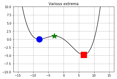
Of the three roots, two correspond to minima—but the left one (blue circle) is greater than the right one (red square), so is it really a minimum? Yes, if we make the distinction between local and global minima. For this problem, the right minimum is the global minimum, while the central root (green star) represents a local maximum (\(f(x)\) is unbounded, i.e., there is no value \(M < \infty\) such that \(|f(x)| < M\) for all possible values of \(x\)). Given the choice, a global optimum is usualy preferred, but for many cases, we’re at best guaranteed a local minimum. There are techniques to increase our chances of finding a global optimum, but that’s outside the present scope!

Solving Unconstrained Optimization Problems

When the Derivative is Available

If we have \(f(x)\) and can evaluate \(f'(x)\), then either Newton’s method or the secant method can be applied to \(f'(x) = 0\). The same goes for multi-variable problems, where the gradient \(\nabla f(\mathbf{x})\) replaces \(f'(x)\), and the hessian matrix \(\mathbf{H}(\mathbf{x})\) replaces \(f''(x)\).

---

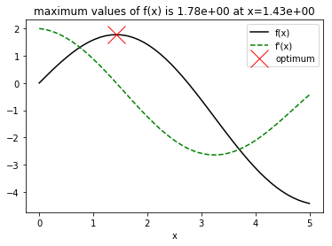
Exercise: Find the value of \(x\) that maximizes the function \(f(x) = 2\sin(x) - x^2/10\) starting with \(x_0 = 2.5\). Then, confirm your result by showing it on a graph of \(f(x)\).

Solution. We can immediately differentiate \(f(x)\) to find \(f'(x) = 2\cos(x) + x/5\) and \(f''(x) = -2\sin(x) + 1/5\). Then, Newton’s method gives

import numpy as np
import matplotlib.pyplot as plt

f = lambda z: 2*np.sin(z) - z**2/10 # objective function
fp = lambda z: 2*np.cos(z) - z/5
fpp = lambda z: -2*np.sin(z) - 1/5

x = 2.5 # initial guess
while abs(fp(x)) > 1e-12:
    x = x - fp(x)/fpp(x)

x_vals = np.linspace(0, 5)
plt.plot(x_vals, f(x_vals), 'k', label='f(x)')
plt.plot(x_vals, fp(x_vals), 'g--', label="f'(x)")
plt.plot(x, f(x), 'rx', ms='20', label='optimum') # X marks the spot...
plt.xlabel('x')
plt.title('maximum values of f(x) is {:.2e} at x={:.2e}'.format(f(x), x))
plt.legend()

<matplotlib.legend.Legend at 0x7f0c80f039e8>

---

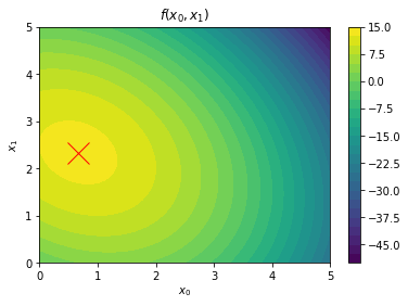
Exercise: Consider the objective function \(f(\mathbf{x}) = ax_0 + bx_1 - (2x_0^2 + x_0 x_1 + 2x_1^2)\). Compute \(\nabla f(\mathbf{x})\) and \(\mathbf{H}(\mathbf{x})\) (which is the jacobian of \(\mathbf{\nabla g}(x)\). Then, for \(a = 5\) and \(b = 10\), determine the values of \(x_0\) and \(x_1\) that maximize \(f(\mathbf{x})\) starting with \(\mathbf{x} = [1, 2]^T\).

Solution:

The gradient is

\[\begin{split}\nabla f(\mathbf{x}) = \left [ \begin{array}{c} \partial f / \partial x_0 \\ \partial f / \partial x_1 \end{array} \right ] = \left [ \begin{array}{c} a - 4 x_0 - x_1 \\ b - 4 x_1 - x_0 \end{array} \right ] \, .\end{split}\]

The hessian matrix is the jacobian matrix for \(\mathbf{\nabla f}(\mathbf{x})\), or

\[\begin{split}\mathbf{H}(\mathbf{x}) = \left [ \begin{array}{cc} \partial \nabla f_0 / \partial x_0 & \partial \nabla f_0 / \partial x_1 \\ \partial \nabla f_1 / \partial x_0 & \partial \nabla f_1 / \partial x_1 \\ \end{array} \right ] = \left [ \begin{array}{c} -4 & -1 \\ -1 & -4 \end{array} \right ] \, .\end{split}\]

Now, apply Newton’s method:

import numpy as np
import matplotlib.pyplot as plt
f = lambda z: 5*z[0] + 10*z[1] - (2*z[0]**2 + z[0]*z[1] + 2*z[1]**2)
gf = lambda z: np.array([5-4*x[0]-x[1],
                        10-4*x[1]-x[0]]) # gradient of f
H = np.array([[-4.0, -1.0],
              [-1.0, -4.0]])

# Apply Newton's method
x = np.array([1.0, 2.0])
while sum(abs(gf(x))) > 1e-8:
    x = x - np.linalg.solve(H, gf(x))

# Plot the results and show where the maximum exists
x0, x1 = np.linspace(0, 5), np.linspace(0, 5)
x0, x1 = np.meshgrid(x0, x1)
plt.contourf(x0, x1, f([x0, x1]), 25)
plt.colorbar()
plt.plot(x[0], x[1], 'rx', ms=20)
plt.xlabel('$x_0$')
plt.ylabel('$x_1$')
plt.title('$f(x_0, x_1)$');

When the Derivative is Unavailable

If we have \(f'(x)\), we can apply Newton’s method to \(f'(x) = 0\). Assuming we don’t, how can we proceed? One option is to adapt the bisection method. Now, the search is not based on the change of the sign of \(f(x)\) but rather it’s magnitude relative to the left and right points. Again, we have to have isolated our (single) target value in some finite range, which may be no easy task (plotting helps). Alternatively, Newton-like methods can be used by approximating both \(f'(x)\) and \(f''(x)\) (or their multi-dimensional analogs) with finite differences.

Using scipy.optimize.minimize

An alternative to Newton’s method is the minimize function in scipy.optimize. From help(minimize), we find

Help on function minimize in module scipy.optimize._minimize:

minimize(fun, x0, args=(), method=None, jac=None, hess=None, hessp=None, bounds=None, constraints=(),
         tol=None, callback=None, options=None)
    Minimization of scalar function of one or more variables.

At a minimum, one must define (1) the function fun to minimize, and (2) an initial guess x0 for the solution. The function minimize returns an object with several attributes, one of which is the solution x. Therefore, if one calls sol = minimize(fun, x0), the solution is sol.x.

---

Exercise: Use minimize to find the maximum of \(f(x) = 2\sin(x) - x^2/10\) starting with \(x_0 = 2.5\).

Solution: Note that any maximization problem can be turned into a minimization problem negating the objective function, i.e., \(f(x)\) becomes \(-f(x)\). Then:

import numpy as np
from scipy.optimize import minimize
f = lambda x: -2*np.sin(x) + x**2 / 10
sol = minimize(f, x0=2.5)
print(sol.x)

[1.42755179]

---

Example: Use minimize to find \(\mathbf{x} = [x_0, x_1]^T\) that minimizes \(f(x) =x_0^2 - x_0 - 2 x_1 - x_0 x_1 + x_1^2\). Use an initial guess of \(x_0 = x_1 = 0\).

Solution:

f = lambda x: x[0]**2 - x[0] -2*x[1] - x[0]*x[1] + x[1]**2
x_initial = [0.0, 0.0]
sol = minimize(f, x0=x_initial)
print(sol.x)

[1.33333353 1.66666666]

Solving Constrained Optimization Problems

Optimization with constraints is a much more challenging problem. Although minimize can be used for such problems, we limit our focus to a specific class of constrained optimization problems known as linear programs. The standard form of a linear program is

\[\min_{\mathbf{x}} \mathbf{c}^T \mathbf{x}\, ,\]

subject to

\[\mathbf{A}_{ub}\mathbf{x} \le \mathbf{b}_{ub} \, ,\]

and

\[\mathbf{A}_{eq}\mathbf{x} = \mathbf{b}_{eq} \, .\]

Note, the objective function is linear, and \(\mathbf{c}\) represents a vector of costs associated with each element of \(\mathbf{x}\).

The ideal tool for solving such problems is scipy.optimize.linprog, for which help provides

linprog(c, A_ub=None, b_ub=None, A_eq=None, b_eq=None, bounds=None, method='simplex', callback=None, options=None)
    Minimize a linear objective function subject to linear
    equality and inequality constraints.

    Linear Programming is intended to solve the following problem form::

        Minimize:     c^T * x

        Subject to:   A_ub * x <= b_ub
                      A_eq * x == b_eq

Here, A_ub and A_eq are two-dimensional arrays, while c, b_ub, and b_eq are one-dimensional arrays.

---

Exercise. Use linprog to find \(\mathbf{x} = [x_0, x_1]^T\) that maximizes \(x_0 + x_1\) subject to the constraints

\[\begin{split}x_0 \ge 0 \\ x_1 \ge 0 \\ x_0 + 2 x_1 \leq 4 \\ 4 x_0 + 2 x_1 \leq 12 \\ -x_0 + x_1 \leq 1 \\\end{split}\]

Solution: Note first that the cost vector \(\mathbf{c}\) should be \([-1, -1]^T\) so that the sum of \(x_0\) and \(x_1\) is maximized. All of the inequality constraints can be cast in \(\mathbf{A}_{ub} \mathbf{x} \le \mathbf{b}_{ub}\) form by noting that if \(x_0 \ge 0\) then \(-x_0 \le 0\). Therefore, these constraints can be written as

\[\begin{split}\left [ \begin{array}{cc} -1 & 0 \\ 0 & -1 \\ 1 & 2 \\ 4 & 2 \\ -1 & 1 \end{array} \right] \left [ \begin{array}{cc} x_0 \\ x_1 \end{array} \right] \leq \left [ \begin{array}{c} 0 \\ 0 \\ 4 \\ 12 \\ 1 \end{array} \right]\end{split}\]

Finally, there are no equality constraints. From here, linprog can be used via

from scipy.optimize import linprog
import numpy as np
c = np.array([-1, -1])
A_ub = np.array([[-1.0, 0.0],
                 [0.0, -1.0],
                 [1.0, 2.0],
                 [4.0, 2.0],
                 [-1.0, 1.0]])
b_ub = np.array([0, 0, 4, 12, 1])
sol=linprog(c, A_ub, b_ub)
print(sol.x) # like minimize, linprog returns an object
             # with attribute x

[2.66666667 0.66666667]

---

Exercise. Suppose the Acme Concrete Company is supplying concrete for three large-scale projects. The company has production facilities in four different locations. Projects 0, 1, and 2 require 250, 400, and 500 cubic meters of concrete each week. Plants A, B, C, and D produce 350, 200, 400, and 450 cubic meters each week. Although the plants, in total, produce more than enough to supply all three projects, the cost to provide the concrete depends on the distance traveled between the plant and the project. The cost per cubic meter to ship from any plant to any project is summarized n the table below:

	0	1
A	10	20
B	15	5
C	25	20
D	30	10

How much should each plant supply to each project? Convert this problem into a linear program, and then use linprog to determine the solution.

---

Further Reading

Checkout out the SciPy documentation on optimization and root finding.