Lecture 20 - Taylor Series and the Root of Numerical Methods

Overview, Objectives, and Key Terms

At this point, the reader is equipped with the basic symbolic tools needed to perform algebraic, differential, and integral operations. In this lecture, another topic from basic calculus is revisited: Taylor series. Along the way, we’ll see how truncated series expansions lead to useful approximations and how those approximations pave the way for numerical methods.

Objectives

By the end of this lesson, you should be able to

• Symbolically compute series expansions of a function
• Explain what is meant by order in the context of series expansions (and numerical approximation)
• Numerically demonstrate that a series expansion of a function provides a good, local approximation

Key Terms

• Taylor series
• Maclaurin series
• \(\mathcal{O}(\Delta^n)\) as order in a different way
• local approximation

Taylor Series

Recall that the Taylor series of a function \(f(x)\) about some point \(x_0\) is defined by

\[\begin{split}\begin{split} f(x) &= f(x_0) + \frac{df}{dx} \Big |_{x = x_0} (x-x_0) + \frac{1}{2} \frac{d^2 f}{dx^2} \Big |_{x = x_0} (x-x_0)^2 + \frac{1}{6}\frac{d^3 f}{d x^3} \Big |_{x = x_0} (x-x_0)^3 + \ldots \\ &= \sum^{\infty}_{n=0} \frac{1}{n!}\frac{d^n f}{dx^n} \Big |_{x=x_0} (x-x_0)^n \end{split}\end{split}\]

When \(x_0\), the series is often called the Maclaurin series.

For the Taylor series for \(f(x)\) about \(x_0\) to exist requires that each derivative of \(f\) exist at \(x_0\). In other words, \(f(x)\) must be infinitely differentiable at \(x_0\). A common phrase in analysis is to say such functions are “well behaved.”

Exercise: Use the differential tools from Lecture 19 to define the \(n\)th term of the Taylor series of \(e^x\) about \(x_0\).

Solution:

import sympy as sy
sy.init_printing()
def nth_term(n):
    x, x_0 = sy.symbols('x x_0')
    return (1/sy.factorial(n)) * sy.diff(sy.exp(x), x).subs(x, x_0) * (x-x_0)**n
nth_term(0), nth_term(1), nth_term(2)

\[$$\left ( e^{x_{0}}, \quad \left(x - x_{0}\right) e^{x_{0}}, \quad \frac{e^{x_{0}}}{2} \left(x - x_{0}\right)^{2}\right )$$\]

Although one could apply such a solution to construct (partial) series representations of a function \(f(x)\), SymPy can do it all at once with the series function:

x, x_0 = sy.symbols('x x_0')
sy.series(sy.exp(x), x, x_0, 3)

\[$$e^{x_{0}} + \left(x - x_{0}\right) e^{x_{0}} + \frac{e^{x_{0}}}{2} \left(x - x_{0}\right)^{2} + \mathcal{O}\left(\left(x - x_{0}\right)^{3}; x\rightarrow x_{0}\right)$$\]

The syntax is easy enough: sy.series(expr, x, x_0, n), where expr is the symbolic expression to expand in series form, x is the independent variable, and x_0 is the point about which the series expansion is defined. In addition, the series will include terms with \((x-x_0)^p\) for \(p < n\).

The result has the same three terms computed explicitly in the solved exercise aboe, but it includes the additional term \(\mathcal{O} \left ( (x-x_0)^3; x\to x_0 \right )\).

We’ll get to what that means in a bit, but for now, we can remove it via

sy.series(sy.exp(x), x, x_0, 3).removeO()

\[$$\frac{e^{x_{0}}}{2} \left(x - x_{0}\right)^{2} + \left(x - x_{0}\right) e^{x_{0}} + e^{x_{0}}$$\]

Exercise Find the first 5 terms of the Maclaurin series for (a) \(f(x) = \sin(x)\), (b) \(f(x) = J_1(x)\) (the Bessel function of the first kind of order 1), and (c) \(\text{erf}(x)\) (the error function).

Exercise Find the two term Taylor series expansion of \((1+x)^a\), known as the binomial approximation. Explore this approximation for different values of \(x\) and \(a\). What can you conclude?

Another Meaning for \(\mathcal{O}\)

Previously, \(\mathcal{O}\) (or big-O) notation was used to define the order of an algorithm. For example, linear search was found to be \(\mathcal{O}(n)\), while binary search was \(\mathcal{O}(\log n)\). In that context, order was proportional to the number of operations (or amount of work) as the problem size grew.

In Taylor series, the \(\mathcal{O}\) means something different: the term \(\mathcal{O} \left ( (x-x_0)^3; x\to x_0 \right )\) formally represents all terms in the series proportional to \((x-x_0)^p\) for \(p \geq 3\). Why capture these terms in one generic \(\mathcal{O}\) term? They all vanish faster than the terms with \(p < 3\) as the different \(x-x_0\) goes to zero.

Note: \(\mathcal{O} \left ((x-x_0)^n\right )\) represents any term proportional to \((x-x_0)^p\) for \(p \geq n\), particularly in the limit that \(x-x_0\) goes to zero.

In practice, the \(\mathcal{O}\) dictates how well a truncated Taylor series can approximate a function \(f(x)\) near \(x_0\). The more terms included in the series, the higher is the power of \((x-x_0)\). As long as \(|x-x_0|\) is small (i.e., \(x\) is near \(x_0\)), higher powers of \(x-x_0\) become vanishingly small.

Exercise: Approximate \(e^x\) using Taylor series approximations with \(n = 1, 2, \ldots 10\) terms about \(x_0 = 0\), evaluate each expression for \(x = 0.1\), and compare to the true value.

Solution:

f = sy.exp(x)
approx = []
exact = sy.exp(0.1)
print('      exact = {:.16f}'.format(exact))
for n in range(1, 11):
    # both sy.series(expr, x) and expr.series(x) work
    f_n = f.series(x, 0, n).removeO()
    print('{:2}th approx = {:.16f}'.format(n, float(f_n.subs(x, 0.1))))

      exact = 1.1051709180756500
 1th approx = 1.0000000000000000
 2th approx = 1.1000000000000001
 3th approx = 1.1050000000000000
 4th approx = 1.1051666666666666
 5th approx = 1.1051708333333332
 6th approx = 1.1051709166666666
 7th approx = 1.1051709180555553
 8th approx = 1.1051709180753966
 9th approx = 1.1051709180756446
10th approx = 1.1051709180756473

The exercise shows that by including additional terms in the sequence the approximation is improved.

Exercise: For \(n = 2 \ldots 4\), plot the \(n\)-term Taylor series approximation for \(e^x\) about the point \(x_0 = 1\) for \(x \in [0, 2]\).

Solution:

import numpy as np
import matplotlib.pyplot as plt
x_plot = np.linspace(0, 2) # prepare x values for plotting
for n in range(2, 5):
    # lambdify the n-term approximation
    f_n = sy.lambdify(x, f.series(x, 1, n).removeO())
    # evaluate that function at the x points for plotting
    f_n_plot = f_n(x_plot)
    # and plot
    plt.plot(x_plot, f_n_plot, label='{}'.format(n))
# plot the exact function for good measure
f_exact = sy.lambdify(x, sy.exp(x))
f_exact_plot = f_exact(x_plot)
plt.plot(x_plot, f_exact_plot, label='exact')
plt.xlabel('x')
plt.legend()
plt.show()

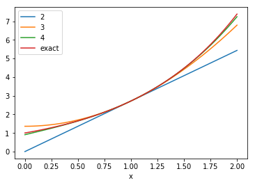
All of the approximations converge to the right value at \(x = 1\) and are good within a small range about the point \(x = 1\). That range grows with \(n\).

Exercise: Modify the solution to the last exercise to show the error, i.e., \(f(x) - f_n(x)\), where \(f_n(x)\) is the \(n\)-term Taylor series approximation.

Exercise: Consider the function \(f(x) = \sin(\sqrt{x})\). How many terms are required to ensure that a \(n\)-term series expansion of this function is accurate to within \(10^{-5}\) (i.e., \(|f(x)-f_n(x)|\)) for all \(x \in [0, 2]\)? Note, there is more than one way to tackle this.

Other Applications

Taylor (and other) series play a major role in function approximation and in development of numerical methods. However, there are other applications in which series expansions can make an otherwise difficult (or impossible) problem easy to solve exactly (or approximately).

Nasty Integrals

Consider the following integral

\[\int^1_0 \cos(x^2) dx\]

Go ahead: try to evaluate it with pen and paper. Stuck? Of course, here’s the answer using sympy.integrate:

sy.integrate(sy.cos(x**2), (x, 0, 1))

\[$$\frac{\sqrt{2} \sqrt{\pi} C\left(\frac{\sqrt{2}}{\sqrt{\pi}}\right) \Gamma{\left(\frac{1}{4} \right)}}{8 \Gamma{\left(\frac{5}{4} \right)}}$$\]

The gamma function is not so rare, but the Fresnel integral (the \(C\)) is pretty exotic. However, consider the first severak non-vanishing terms of the Taylor series of the integrand \(\cos(x^2)\):

sy.cos(x**2).series(x, 0, 20)

\[$$1 - \frac{x^{4}}{2} + \frac{x^{8}}{24} - \frac{x^{12}}{720} + \frac{x^{16}}{40320} + \mathcal{O}\left(x^{20}\right)$$\]

In other words, the \(i\)th nonzero term is \((-1)^i\frac{x^{4i}}{2i!}\) for \(i = 0, 1, \ldots\). Each term can be integrated over the range (recall, the integral of a sum is the sum of the integrals), leading to terms of the form \((-1)^i\frac{1}{(4i+1)\cdot 2i!}\) (\(i = 0, 1, \ldots\)). The result is a convergent series that can be evaluated directly using Sum and limit, similar to what was done in Lecture 19.

Exercise: Set up this Sum and evaluate the limit. Is it consistent with what you get upon numerically evaluating the integral above?

Exercise: Repeat the exercise for \(\int^x_0 e^{-z^2} dz\). What does application of sympy.simplify to the final limit yield?

Stability of Nonlinear Systems

Future work!

Further Reading

None for now.