Numerical Differentiation
Overview, Objectives, and Key Terms
From Lecture 1 through Lecture 17, the focus has been squarely on the fundamentals of programming, with some basic numerical tools (like numerical arrays and plotting) and best practices (like unit testing) included along the way. Our focus now shifts to the use of programming to solve problems numerically. We still need the basic tools we’ve acquired (loops, functions, etc.), but our purpose is in application. In this lesson, we’ll review the basics of Taylor series and how they can be used to define finite-difference approximations for derivatives. We’ll need these later in Root Finding and Numerical Solution of BVPs.
Objectives
By the end of this lesson, you should be able to
- Derive finite-difference approximations for first- and second-order derivatives using Taylor series.
- Numerically/graphically/symbolically demonstrate that the error of an \(n\)th-order approximation as \(\Delta \to 0\) exhibits the right behavior.
Key Terms
- finite difference
- forward difference
- backward difference
- central difference
- truncation error
- absolute error
- order of error
- first-order approximation
- second-order approximation
- \(n\)th-order approximation
If, in the beginning, \(\Delta\) didn’t go to 0...
Recall that the derivative of \(f(x)\) is
Here, \(h\) (the ubiquitous “step” used in calculus books around the world) is swapped for \(\Delta\) (a better symbol that represents “small change”). What if that limit is not taken and, instead, a “small” value of \(\Delta\) is used? The result is our first finite-difference approximation, the forward difference:
This is called the forward difference approximation because \(f'(x)\) depends on information (1) at point \(x\) and (2) to the right (or forward) of \(x\) at \(x+\Delta\). Intuition suggests that this approximation improves with smaller \(\Delta\).
An equally valid approximation is the backward difference:
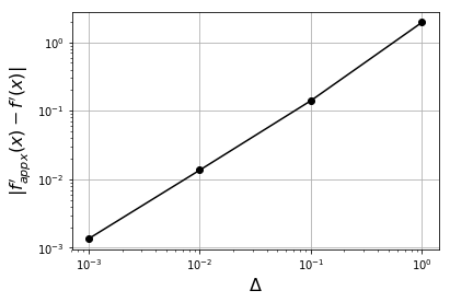
Exercise: Use the forward-difference approximation to approximate the derivative of \(e^x\) at \(x = 1\) for \(\Delta = 1\), \(0.1\), \(0.01\), and \(0.001\). Plot the absolute error as a function of \(\Delta\) using a log-log scale.
Solution:
In [2]:
import numpy as np
import matplotlib.pyplot as plt
# point at which derivative is to be evaluat
x = 1.0
# define reference derivative (fp for "f prime")
fp_ref = np.exp(x)
# define the step sizes to use
Delta = np.logspace(0, -3, 4)
# initialize the approximate derivative
fp_appx = np.zeros(len(Delta))
# compute the approximate derivative for each value of Delta
for i in range(len(Delta)):
    fp_appx[i] = (np.exp(x+Delta[i])-np.exp(x))/Delta[i]
# plot using a log-log scale
plt.loglog(Delta, abs(fp_appx-fp_ref), 'k-o')
plt.xlabel('$\Delta$', fontsize=16)
plt.ylabel("$|f_{appx}'(x)-f'(x)|$", fontsize=16)
plt.grid(True)
plt.show()
Exercise: Repeat the previous exercise but use the backward difference. Do you observe any difference?
Back to Order
The solved exercise above suggests that the forward-difference approximation yields a better approximation as \(\Delta\) grows smaller, but how much better? To answer this, we consider the Taylor series for \(f(x+\Delta)\) about the point \(x\):
By isolating \(f'(x)\) on one side, we have
In other words, the forward difference leaves out terms proportional to \(\Delta\) and higher powers of \(\Delta\). Moreover, as \(\Delta\) shrinks, \(\Delta \gg \Delta^p\) for \(p > 1\). The terms left out represent the truncation error, and because this error goes as \(\Delta^1\) for small \(\Delta\), the order of the error is 1, i.e., the forward-difference approximation is a first-order approximation.
Exercise: Show that the backward-difference approximation is also first order.
Can we do better than first order? It turns out that we can. Consider the following Taylor series:
Subtraction of this series from the one above for \(f(x+\Delta)\) leads to
or
This latter approximation for \(f'(x)\) is a central difference and is a second-order approximation because \(\Delta\) is raised to the second power.
Note: Forward and backward differences yield first-order approximations to \(f'(x)\), while the central difference yields a second-order approximation for \(f'(x)\).
Exercise: Consider the Taylor series for \(f(x-\Delta)\), \(f(x+\Delta)\), \(f(x-2\Delta)\), and \(f(x+2\Delta)\). Try to develop a fourth-order approximation for \(f'(x)\) that involves these four values of \(f\).
Exercise: Consider a function \(f(x)\) for which you are given values only at \(x = i\Delta\) for \(i = 0, 1, 2, \ldots\) for small \(\Delta\). Suppose that some application requires that you evaluate \(f(x)\) at some middle point \((i+1/2)\Delta\). Of course, the natural thing to do is average the two adjacent values at \(i\Delta\) and \((i+1)\Delta\). What order is this averaging approximation?
Exercise: Apply the central difference to the function \(f(x) = \sin(2x - 0.17) + 0.3 \cos(3.4x + 0.1)\) at \(x = 0.5\). Plot the error for \(\Delta = 10^{-1}, 10^{-2}, \ldots, 10^{-7}\).
Approximating the Second Derivative
So far, the finite differences developed represent approximations to the first derivative, \(f'(x)\). Approximations for the second derivative can be derived in a similar fashion. Consider again the Taylor series for \(f(x+\Delta)\) and \(f(x-\Delta)\). Whereas these series were subtracted to yield the central-difference approximation for \(f'(x)\), they can insteady be added to yield the following:
where both the \(f'\) and \(f'''\) terms cancel. By isolating \(f''(x)\), we have
which is the central-difference approximation for the second derivative. Like the central-difference approximation for the first derivative, the truncation error is second order.
By the way, how can we establish order? In fact, Lecture 14 and Lecture 15 introduced numerical experiments for searching and sorting to establish an algorithm’s order. Although “order” means something different here, the technique is similar: we test the approximation for different values of \(\Delta\) and see whether the error goes as \(\Delta\) or \(\Delta^2\) or something else entirely. By “see”, I mean literally: use a graphic!
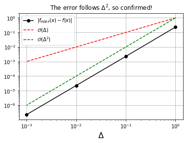
Exercise: Confirm graphically that the central-difference approximation for the second derivative is, in fact, second order. Use \(f(x) = e^x\) for demonstration.
Solution: I set us up for success with the last solved exercise, which is adapted here.
In [2]:
import numpy as np
import matplotlib.pyplot as plt
x = 1.0
fpp_ref = np.exp(x) # fpp for "f prime prime"
Delta = np.logspace(0, -3, 4)
fpp_appx = np.zeros(len(Delta))
for i in range(len(Delta)):
    fpp_appx[i] = (np.exp(x+Delta[i])-2*np.exp(x)+np.exp(x-Delta[i]))/Delta[i]**2
plt.loglog(Delta, abs(fpp_appx-fpp_ref), 'k-o', label='$|f_{appx}''(x)-f''(x)|$')
plt.loglog(Delta, Delta, 'r--', label='$\mathcal{O}(\Delta)$')
plt.loglog(Delta, Delta**2, 'g--', label='$\mathcal{O}(\Delta^2)$')
plt.xlabel('$\Delta$', fontsize=16)
plt.legend()
plt.grid(True)
plt.title('The error follows $\Delta^2$, so confirmed!')
plt.show()
Finite-Difference Approximations of Arbitrary Order
The finite-difference approximations explored were identified pretty easily by manipulating the Taylor series of a function. Approximations that are higher order or that can be used for higher derivatives are somewhat more challenging to develop.
Simple Rules
Generally, approximations that use values of \(f\) at more values of \(x\) (e.g., \(x-\Delta\) and \(x+\Delta\)) are better than those that use fewer.
A more specific rule-of-thumb: an \(n\)th-order approximation for the \(m\)th derivative requires that \(f\) be evaluated at \(n+m-1\) evenly-spaced \(x\) values if those values are symmetric about \(x\) (e.g., \(x-\Delta\) and \(x+\Delta\) as used for the central difference) or \(n+m\) points, if the points are not symmetric about \(x\) (e.g., \(x-\Delta\) and \(x\) as used for the backward difference).
Exercise: Does the backward-difference approximation for \(df/dx\) follow this rule?
Solution: The backward-difference approximation for the first derivative (\(m=1\)) is first order (\(n=1\)). The points are not symmetric about \(x\). Hence, the rule requires \(m+n = 2\) points, consistent with the approximation.
Exercise: Does the forward-difference approximation for \(df/dx\) follow this rule?
Exercise: Does the central-difference approximation for \(df/dx\) follow this rule?
Exercise: Does the central-difference approximation for \(d^2f/dx^2\) follow this rule?
Further Reading
None for now.