Numerical Integration

Overview, Objectives, and Key Terms

In Numerical_Differentiaton, finite-difference approximations were developed and used to evaluate derivatives numerically. In this lecture, we’ll explore and implement our own numerical methods for evaluation of integrals. We’ll also use the SciPy module for the first time, which provides its own set of tools for numerical integration.

Objectives

By the end of this lesson, you should be able to

• Evaluate definite integrals numerically using left- and right-sided Riemann sums, the mid-point rule, and the trapezoid rule.
• Evaluate definite integrals numerically using the built-in functions of scipy.integrate
• Establish the order of an integration scheme using numerical, graphical, or symbolic means.

Key Terms

• Riemann sum
• left-sided Riemann sum
• right-sided Riemann sum
• mid-point rule
• trapezoid rule
• scipy.integrate
• scipy.integrate.quad
• \(n\)th-order approximation

Riemann Sums in Practice

For derivatives, we took a limit of a finite difference for an exact answer but stopped that limit for a sufficiently small \(\Delta\) to ensure a reasonable estimate. For the first derivative, we saw the first-order forward and backward schemes along with the second-order central difference scheme.

For integrals, we have analogs to these choices. You may remember the following formal definition for a definite integral:

\[\int^b_a f(x) dx = \lim_{n \to \infty} \sum^{n}_{i=1} f(i (b-a)/n + a) (b-a)/n\]

Here, the sum is a Riemann sum (specifically a right-sided sum). Integrals are areas under curves, and Riemann sums approximate those areas by rectangles. Just as for derivatives, we don’t take the limit but let \(n\) be a finite number. Moreover, we have different Our numerical options depending on how we define the rectangles of the Riemann sum.

Let’s look at this concretely for \(f(x) = x^2\) over \(x\in[0, 1]\) with \(n=5\):

import riemann_sum_plots
riemann_sum_plots.right_sided_sum()

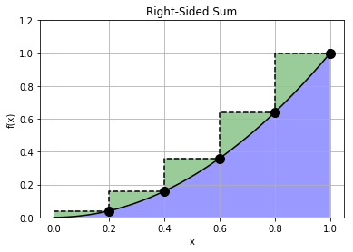
Notice that the height of a rectangle is equal to the function evaluated at the rectangle’s right \(x\) coordinate. We call such a sum a right-sided Riemann sum. For this particular function, this right-sided sum leads to some significant over estimation.

If instead we defined our sum to be

\[S =\frac{b-a}{n} \sum^{n}_{i=1} f \Bigg ( \frac{ (i-1)(b-a) }{n} + a \Bigg )\]

the picture becomes

riemann_sum_plots.left_sided_sum()

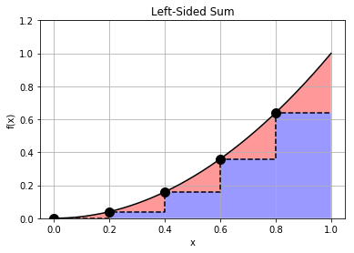
Here, the rectangle height is based on the function evaluated at its left side, making this a left-sided Riemann sum. Just as the right-sided sum overestimates the integral, the left-sided sum underestimates the integral.

---

Exercise: Given the points \(x = [0, 2/3, 4/3, 2]\) and corresponding values \(y = [1, 3/5, 3/7, 1/3]\), estimate \(\int^2_0 y(x)dx\) using the right-sided sum and left-sided sum. What is the true value (assuming \(y = (x+1)^{-1}\))?

---

Exercise: Consider the following two columns of data:

\(x\)	\(\sqrt{x}\)
0.0000	0.0000
0.3333	0.5774
1.0000	1.0000
1.5000	1.2247
2.0000	1.4142

Estimate \(\int^2_0 f(x) dx\) using the right-sided sum and left-sided sum. Note that the \(x\) points are not evenly spaced.

---

Beyond the One-Side Sums

Can we do better? Remember, I said that the forward, backward, and central finite-difference approximations have analogous Riemann sums. Here, take the right- and left-sided sums to be like the forward and backward differences. If you hadn’t noticed, the central difference is nothing but an average of the forward and backward differences:

\[\frac{1}{2} \Bigg ( \frac{f(x+h)-f(x)}{h} + \frac{f(x)-f(x-h)}{h} \Bigg ) = \frac{f(x+h)-f(x-h)}{2h}\]

so we might expect something similar for the Riemann sums. There are two possibilities. First, we can evaluate the rectangle heights at the average value of its \(x\) coordinates, i.e.,

\[S = \frac{b-a}{n} \sum^{n}_{i=1} f \Bigg ( \frac{ (i-1/2)(b-a) }{n} + a \Bigg )\]

for which the picture becomes

riemann_sum_plots.midpoint_sum()

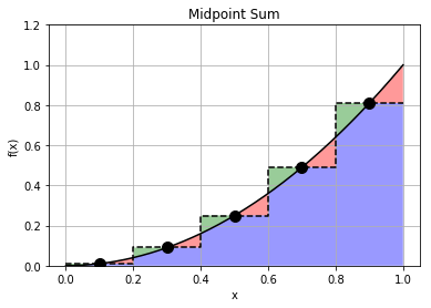
This method is often called the midpoint rule, and it’s probably my favorite integration scheme because it’s pretty accurate and dirt simple to implement.

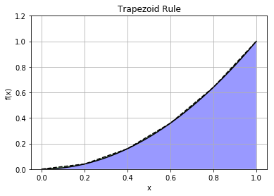
The alternative is to average the right- and left-sided sums, which leads to

\[\begin{split}\begin{split} S &= \frac{b-a}{2n} \Bigg [ \sum^{n}_{i=1} f \Bigg ( \frac{ (i)(b-a) }{n} + a \Bigg ) + \sum^{n}_{i=1} f \Bigg ( \frac{ (i-1)(b-a) }{n} + a \Bigg ) \Bigg ] \\ &= \frac{b-a}{2n} \Bigg [ f(a) + f(b) + \sum^{n-1}_{i=1} f \Bigg ( \frac{ i(b-a) }{n} + a \Bigg ) \Bigg ] \end{split}\end{split}\]

If you consider this carefully, the resulting geometric picture turns rectangles into trapezoids (because the average of the area of two rectangles of heights \(y(x_1)\) and \(y(x_2)\) that share the same \(x\) coordinates \(x_1\) and \(x_2\) is equal to the area of the trapezoid whose coordinates include \((x_1, y_1)\) and \((x_2, y_2)\)), and the method is known as the trapezoid rule. (It’s those pesky end-point terms \((a)\) and \(f(b)\) that make this rule just a hair less convenient to apply in some cases, so I always stick to the midpoint rule when I can!)

riemann_sum_plots.trapezoid_rule()

For a function \(f(x)\) with sufficiently nice properties (beyond our scope), it’s not too difficult to estimate the error associated with these integrals as \(\Delta = (b-a)/n\) goes to zero (or equivalently, \(n \to \infty\). However, I’ll skip giving away the answers and let you determine these properties by numerical experiments in the homework!

Finally, the integration rules just explored represent the simplest possible Newton-Cotes formulas. The basic idea of Newton-Cotes integration is that a function \(f(x)\) is assumed to be piece-wise polynomial in finite ranges and evaluated at evenly-spaced points \(x_i\). Left-sided sums, right-sided sums, and and the midpoint rule take \(f(x)\) to be constant between adjacent points \(x_i\) and \(x_{i+1}\), while the trapezoid rule assumes \(f(x)\) is linear between adjacent points. If \(f(x)\) is assumed to be quadratic between \(x_i\) and \(x_{i+2}\), the result is Simpson’s rule (another favorite of mine).

---

Exercise: Suppose you accessed your fancy phone’s accelerometer log and extracted the following accelerations (in m/s\(^2\)) and times (in s):

a = 0, 0.1, 0.3, -0.2, 0.1
t = 2, 4, 6, 8, 10

Estimate how far you went in those 8 seconds using the trapezoid rule. ***

Exercise: Recall that the incremental work \(\delta W\) done by an expanding gas is given by \(\delta W = p \delta V\), where \(p\) is pressure and \(\delta V\) is the change in volume. Consider the following table of measured pressures (MPa) for several volumes (cm ³) during the expansion of the gas within an internal combustion engine.

\(p\)	\(V\)
15.6835	79.8508
12.7127	88.6913
9.3703	103.3057
6.5612	123.4549
4.5031	149.0202
2.0138	222.8411

Estimate the work performed by the gas using the trapezoid rule.

---

Exercise: Revisit the last exercise by determinging the \(n\) that satisfies \(pV^n = c\) for some constant \(c\). Then, using the same measured data, apply the midpoint rule to estimate the work done by the gas.

---

What About Accuracy?

As was done for the finite-difference methods, it is possible to determine the order of various numerical integration rules. The basic idea is to observe the (absolute) error between an exact, reference value for an integral and the approximation of that integral for various step sizes \(\Delta\).

---

Exercise: Determine whether the right-sided sum is first order or second order using the definite integral \(\int^1_0 e^x dx = e - 1\) as a test case.

Solution:

import numpy as np
import matplotlib.pyplot as plt

def right_sided_sum(f, a, b, n):
    """Approximate the integral of f over [a, b] using
       the right-sided sum and n evenly spaced points."""
    x = np.linspace(a, b, n+1)[1:]
    return np.sum(f(x))*(x[1]-x[0])

# reference integral value
I_ref = np.exp(1) - 1.0
# number of points to use in each sum
n_vals = 2**np.arange(1, 10)
# initialize the approximate integrals
I_appx = np.zeros(len(n_vals))
for i in range(len(n_vals)):
    I_appx[i] = right_sided_sum(np.exp, 0, 1, n_vals[i])
# absolute error
I_err = abs(I_appx-I_ref)
# Delta = (b-a)/(n+1)
Delta = 1/(n_vals+1)
# Plot the error along with linear and quadratic forms
plt.loglog(Delta, I_err, 'k', label='error')
plt.loglog(Delta, Delta, 'r--', label='$\mathcal{O}(\Delta)$')
plt.loglog(Delta, 10*Delta**2, 'b-.', label='$\mathcal{O}(\Delta^2)$')
plt.xlabel('$\Delta$')
plt.legend()
plt.show()

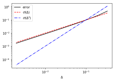
Surely, the error is much closer to the \(\mathcal{O}(\Delta)\) term and, hence, the right-sided sum is first order.

---

Exercise: Determine the order of the left-sided sum, midpoint rule, and trapezoid rule. You may use the definite integral \(\int^1_0 e^x dx = e - 1\) as a test case.

---

Using scipy.integrate

As alternatives to the simple schemes explored above, several integration schemes are provided by scipy.integrate. SciPy is a large collection of open-source, Python tools for numerical and other scientific computing. For example, NumPy is a major component of SciPy but is often used as a standalone package (as are Matplotlib and SymPy).

Other schemes exist for multidimensional integration.

SciPy offers several integrations schemes in its scipy.integrate module. However, the best choice for most problems is the quad function, which is based on a Gauss-Kronrod scheme. Here it is in action:

from scipy.integrate import quad
quad(np.exp, a=0, b=1)

(1.7182818284590453, 1.9076760487502457e-14)

By default, quad returns both the approximate integral and the estimated absolute error. Here, that error is ridiculously small (close to machine precision). For many problems, that’s all that one needs to do in order to compute an integral. However, quad does have a variety of optional input parameters, and, as always, you may learn more by executing help(quad).

Other functions in scipy.integrate that are of interest include trapz (the trapezoid rule) and simps (Simpson’s rule). Use of help on each function is recommended, as examples are provided in the documentation.

Further Reading

None.