Basic Operators and Built-In Functions

Overview, Objectives, and Key Terms

In this lesson, we’ll continue our study of basic types from Lecture 1, incorporating operators (arithmetic and otherwise) along with some very useful built-in functions. By the end, we’ll construct our very first (albeit, simple) program.

Objectives

By the end of this lesson, you should be able to

• add, subtract, multiply, and divide two quantities
• use the help() function to understand how to use another function
• use dir() and the variable explorer to see defined variables and their values
• explain the difference between statement and expression
• write a short, well-commented program

Key Terms

• statement
• expression
• variable explorer
• keywords
• import
• math module
• dir()
• help()
• print()
• type()
• +, -, *, /, **, //, ^
• flowchart
• comments and the # symbol

# These two lines modify the Jupyter notebook behavior
# a bit.  Now, all lines in a cell with only an expression
# will be printed, not just the last one.  I've included
# an example.  This feature lets us use just one cell for
# lots of simple output without using print
from IPython.core.interactiveshell import InteractiveShell
InteractiveShell.ast_node_interactivity = "all"

a = 1
b = 2
a # a will be printed
b # b will also be printed

1

2

Python Operators

In Lecture 1, we saw several examples of the form a = 1, where the variable a is assigned the value 1. Here, = is the assignment operator. The entire line of code a = 1 is a statement. A statement represents an instruction that is performed by the computer (and, in this case, the Python interpreter).

Arithmetic Operators

There are several other operators in the Python language, including those known as the arithmetic operators summarized in the table below. In the table, a and b can assumed to be int variables (though all but the last operator can be used for float variables). One example is the addition operator, which can be used as a + b. This fragment of code is an expression, which is any combination of values, operators, and function calls that can be evaluated, i.e., has a value. Expressions are distinct from statements. For example, a + b is an expression (defines a value), but c = a + b is a statement (in this case, assignment of a value to a variable c).

symbol	example use	definition
+	a + b	add b to a
-	a - b	subtract b from a
*	a * b	multiply a by b
/	a / b	divide a by b
//	a // b	divide a by b using integer arithmetic
%	a % b	remainder of a / b
**	a**b	raise a to the power of b
^	a^b	bitwise exclusive or

The first four operators are pretty straightforward and are the same symbols used in a variety of programming languages and other tools (e.g., common spreadsheets). The remaining four warrant some elaboration. The operator // corresponds to integer division. Integer division rounds the final result down to the nearest integral value. Here’s a quick example for illustration:

a = 4
b = 3
print(a/b)
print(a//b)

1.3333333333333333
1

The first value printed is what we expect (i.e., 4/3 cast in decimal notation), while the second printed value is obviously rounded.

Warning: In case you ever use Python 2, / was implemented as integer division by default for a and b of type int.

The symbol % represents the modulus (or remainder) operation. Often written \(a \mod b\), the modulus operation yields the remainder after integer division. For example, \(10/3\) has a remainder of 1, so \(10 \mod 3 = 1\) and, in Python, that is written as 10 % 3.

The final two operators listed may also cause some confusion. Here, ** represents the exponentiation (or power) operation. In some languages/tools (notably MATLAB and Excel), ^ is the symbol for exponentiation, but in Python, ^ is for the probably foreign-sounding bitwise exclusive or (and, hence, is not actually an arithmetic operator). To understand bitwise operators, we’ll need to dive into binary numbers (but we’ll skip that for the moment).

Warning: Do not use ^ when you want to take a to the power of b. Instead, use a**b.

Sometimes, an arithmetic operator can be used in situations that do not involved numbers. For instance, strings can be concatenated (i.e., joined) using addition:

s = "go "
t = "wildcats!"
u = s + t
u

'go wildcats!'

Strings can also be multiplied by integers, which leads to a repeated sequence of the original string. For example, we could turn 'xo' into 'xoxoxo' using

'xo' * 3 # or 3 * 'xo'

'xoxoxo'

Assignment Operators

Corresponding to each arithmetic operator is a combined arithmetic and assignment operator. Recall that the assignment operator = can be used to assign the value of b to the variable a, i.e., a = b. However, perhaps we have a defined already and we want to increase it by b. We could execute a = a + b. However, a shorter and logically equivalent approach is to execute a += b. The table below summarizes all of these combined assignment operators.

symbol	example use	definition
=	a = b	assign the value of a to the variable a
+=	a += b	equivalent to a = a + b
-=	a -= b	equivalent to a = a - b
*=	a *= b	equivalent to a = a * b
/=	a /= b	equivalent to a = a / b
//=	a //= b	equivalent to a = a // b
%=	a %= b	equivalent to a = a % b
**=	a = a**b	equivalent to a = a**b

Relational Operators

In Lecture 1, the bool type was introduced, with bool variables having one of two values True or False. Sometimes, we need to know whether some expression is either True or False. For instance, is it true that “a is greater than b?” To evaluate whether or not this is true, we need a relational operator, in this case, the greater than operator >. Here it is in action:

a > b

True

Of course, we had defined a = 4 and b = 3 above, so a it is true that a is greater than b. Also note a useful behavior of interactive Python (whether using IDLE or IPython): whenever a line of code is an expression and not a statement, evaluation of that line of code leads to output that contains the value of the expression. Here, a > b is the expression, and True is its value.

Note: Executing a line of code containing only an expression in IDLE or IPython leads to an output line containing the value of that expression.

The table below summarizes the relational operators.

symbol	example use	definition
==	a == b	a equal to b yields True
!=	a != b	a not equal to b yields True
>	a > b	a greater than b yields True
>=	a >= b	a greater than or equal to b yields True
<	a < b	a less than b yields True
<=	a <= b	a less than or equal to b yields True

Logical Operators

Related to relational operators are the logical operators not, and, and or. When applied to any boolean value, the not operator flips the original value. In other words, not True is equal to False, and not False is equal to True. The not operator can be used on any expression whose value is a bool:

v = 1 > 2 # surely False
not v

True

One can also apply the not operator to values that are not bool values but that can be converted to bool values:

v = 1 # an int, not a bool, but logically equivalent to True
not v

False

The and and or operators are used in the form a and b and a or b, respectively. If a and b are bool variables, the and and or operators work just like we’d expect: and requires that both a and b are True for the entire expression to be True, while or leads to True for three cases:

1. a is True and b is False
2. a is False and b is True
3. a is True and b is False

In other words, a or b is False only if a is False and b is False.

---

Exercise: Confirm the values of all combinations of a and b where a and b are bool values by evaluating each expression in Python.

Solution:

a = True
b = True
a and b

True

a = True
b = False
a and b

False

a = False
b = True
a and b

False

a = False
b = False
a and b

False

---

Exercise: Confirm all the values of all combinations of a and b where a and b are bool values.

---

When a and b are not bool variables, the behavior of and and or is a bit more complex (but consistent with the behavior observed above). Consider specifically the case a and b. To evaluate this expression, a is first converted into a bool value (and if that’s not possible, an error would arise). Do non-bool values have an associated bool value? In many cases, yes. For example, the integer 0 is logically False, while any other integer is True:

bool(0)
bool(1234)
bool(-23)

False

True

True

The bool value of a str value is False only for the empty string '':

bool('')
bool('not empty')

False

True

When a and b is evaluated, the value is the first False or False-equivalent (e.g., '') encountered. Otherwise, the value is the last True or True-equivalent (e.g., 1) encountered. When a or b is evaluated, the value is the first True-equivalent encountered or the second False-equivalent encountered.

---

Exercise: Evaluate the following logical expressions and explain each result.. Try to do so without using Python first, and then check your answer by evaluating the expression in Python.

• 1 and 0
• '' and 0.0
• 1 and 'a'
• 1 or 'a'
• 0 or 'a'
• 0 or ''

Solution: For 1 and 0, note that 1is logically equivalent to True, but 0 is logically equivalent to False. Hence, the result is 0, as is easily verified:

1 and 0

0

Consider now '' and 0.0. Both '' and 0.0 are logically equivalent to False. Since '' is the first value, it makes the and expression False and, hence, it’s the final result:

'' and 0.0

''

Finally, consider 1 and 'a'. Both 1 and 'a' evaluate to True. Hence, the and expression is True, and it’s the second value 'a' that makes it so:

1 and 'a'

'a'

The other expressions can be analyzed in similar fashion. Evaluate them in Python to double-check your result!

---

Order of Operations

Several arithmetic and other operators can be used in one expression, and the order in which they are applied is important to understand. The basic arithmetic operators are applied using the same rules applied in mathematics: exponentiation is performed before multiplication and division, and addition and subtraction happen last. For example, consider \(2 + 3 \times 4^2\). First, \(4^2\) is evaluated, leaving \(2 + 3\times 16\). Then \(3\times 16\) is evaluated, leaving \(2 + 48\). Finally, the addition is evaluated, leaving \(50\).

One way to modify the order of operations is by using parentheses, e.g., \((2 + 3)\times 4^2\), which is evaluated as \(5 \times 4^2 = 5 \times 16 = 80\). Just to verify:

2 + 3 * 4**2

50

(2 + 3) * 4**2

80

The order in which operations are performed can be categorized as follows, from first to last evaluated:

1. ()‘s
2. *, /, //, and %
3. +, -
4. <, <=, etc.
5. not
6. and
7. or

This list indicates that parentheses are evaluated first, while the or operator is evaluated last.

---

Exercise: Evaluate the following arithmetic expressions by hand (and then check with Python):

• 17 / 2 * 3 + 2
• 2 + 17 / 2 * 3
• 19 % 4 + 15 // 2  * 3
• (15 + 6) - 10 * 4
• 17 / 2 % 2 * 3**3

---

Exercise: Evaluate the following expressions by hand (and then check with Python):

• 2 * 3 < 4
• 3 < 6 < 9
• 3 < 6 <= 1 + 2 + 3

---

Exercise: What is the value of the the expression 3 > 4 or 5?

Solution: You might be tempted to read this expression as “is 3 greater than either 4 or 5?” Of course, 3 is less than both 4 or 5. However, the order of operations requires the 3 > 4 to be evaluated first. Broken down step by step, the evaluation is

0. 3 > 4 or 5
1. False or 5 (because 3 > 4 is False)
2. 5 (the final result, which you should verify!)

---

Exercise: The rules of operation order can trick the most seasoned programmers. Come up with your own expressions involving at least three types of operators and try to stump your friends!

---

Exploring Built-In Functions

Armed with the operators described above, you’ve got the start to a powerful, interactive calculator using Python. What we need next is some of the typical mathematical functions. We’ll get to defining our own functions later on, but Python has several built-in functions that are useful, we can get access to a whole bunch of useful functions just by using powerful import statements.

You’ve actually already seen your first function: print. A function has a name (e.g., print) and accepts zero, one, or more arguments enclosed in parentheses. For example, we can call the print function in several different ways:

print("Hello, world") # one argument, a str
print(1, 2, 3) # three, int arguments
print("What's my age again?", 18) # mixed arguments (and, I'm lying)

Hello, world
1 2 3
What's my age again? 18

Notice: Any call to a function must include parentheses.

help()

A second function everyone ought to know is help. Let’s call it, and when it prompts us for further input, let’s enter “symbols.” After that, we’ll enter “quit.”

help() # remember, parentheses are needed even if we have nothing in them!

Welcome to Python 3.6's help utility!

If this is your first time using Python, you should definitely check out
the tutorial on the Internet at https://docs.python.org/3.6/tutorial/.

Enter the name of any module, keyword, or topic to get help on writing
Python programs and using Python modules.  To quit this help utility and
return to the interpreter, just type "quit".

To get a list of available modules, keywords, symbols, or topics, type
"modules", "keywords", "symbols", or "topics".  Each module also comes
with a one-line summary of what it does; to list the modules whose name
or summary contain a given string such as "spam", type "modules spam".

help> symbols

Here is a list of the punctuation symbols which Python assigns special meaning
to. Enter any symbol to get more help.

!=                  *=                  <<                  ^
"                   +                   <<=                 ^=
"""                 +=                  <=                  _
%                   ,                   <>                  __
%=                  -                   ==                  `
&                   -=                  >                   b"
&=                  .                   >=                  b'
'                   ...                 >>                  j
'''                 /                   >>=                 r"
(                   //                  @                   r'
)                   //=                 J                   |
*                   /=                  [                   |=
**                  :                   \                   ~
**=                 <                   ]

help> quit

You are now leaving help and returning to the Python interpreter.
If you want to ask for help on a particular object directly from the
interpreter, you can type "help(object)".  Executing "help('string')"
has the same effect as typing a particular string at the help> prompt.

We can also use help directly to learn about a variable or function. For example, how can we use print? Let’s use help to figure that out:

help(print)

Help on built-in function print in module builtins:

print(...)
    print(value, ..., sep=' ', end='\n', file=sys.stdout, flush=False)

    Prints the values to a stream, or to sys.stdout by default.
    Optional keyword arguments:
    file:  a file-like object (stream); defaults to the current sys.stdout.
    sep:   string inserted between values, default a space.
    end:   string appended after the last value, default a newline.
    flush: whether to forcibly flush the stream.

When we work in IPython, another way to obtain help is by using the question mark ? placed immediately after whatever name about which we need information, e.g., print?. The output is slightly different in format but equivalent to the output of help.

dir and type

Another very useful function is dir. If we call it without arguments, it gives us the following:

dir()

['In',
 'InteractiveShell',
 'Out',
 '_',
 '_10',
 '_11',
 '_12',
 '_13',
 '_14',
 '_15',
 '_16',
 '_17',
 '_18',
 '_19',
 '_2',
 '_4',
 '_5',
 '_6',
 '_7',
 '_8',
 '_9',
 '__',
 '___',
 '__builtin__',
 '__builtins__',
 '__doc__',
 '__loader__',
 '__name__',
 '__package__',
 '__spec__',
 '_dh',
 '_i',
 '_i1',
 '_i10',
 '_i11',
 '_i12',
 '_i13',
 '_i14',
 '_i15',
 '_i16',
 '_i17',
 '_i18',
 '_i19',
 '_i2',
 '_i20',
 '_i21',
 '_i22',
 '_i23',
 '_i3',
 '_i4',
 '_i5',
 '_i6',
 '_i7',
 '_i8',
 '_i9',
 '_ih',
 '_ii',
 '_iii',
 '_oh',
 'a',
 'b',
 'exit',
 'get_ipython',
 'quit',
 's',
 't',
 'u',
 'v']

This output shows all of the names (variables and functions) currently defined, including a and b from the examples above. Most of the items shown are not important for users, but __builtin__ provides us a way to see the names of all functions and other things defined by default. Again, we turn to dir:

dir(__builtin__)

['ArithmeticError',
 'AssertionError',
 'AttributeError',
 'BaseException',
 'BlockingIOError',
 'BrokenPipeError',
 'BufferError',
 'BytesWarning',
 'ChildProcessError',
 'ConnectionAbortedError',
 'ConnectionError',
 'ConnectionRefusedError',
 'ConnectionResetError',
 'DeprecationWarning',
 'EOFError',
 'Ellipsis',
 'EnvironmentError',
 'Exception',
 'False',
 'FileExistsError',
 'FileNotFoundError',
 'FloatingPointError',
 'FutureWarning',
 'GeneratorExit',
 'IOError',
 'ImportError',
 'ImportWarning',
 'IndentationError',
 'IndexError',
 'InterruptedError',
 'IsADirectoryError',
 'KeyError',
 'KeyboardInterrupt',
 'LookupError',
 'MemoryError',
 'ModuleNotFoundError',
 'NameError',
 'None',
 'NotADirectoryError',
 'NotImplemented',
 'NotImplementedError',
 'OSError',
 'OverflowError',
 'PendingDeprecationWarning',
 'PermissionError',
 'ProcessLookupError',
 'RecursionError',
 'ReferenceError',
 'ResourceWarning',
 'RuntimeError',
 'RuntimeWarning',
 'StopAsyncIteration',
 'StopIteration',
 'SyntaxError',
 'SyntaxWarning',
 'SystemError',
 'SystemExit',
 'TabError',
 'TimeoutError',
 'True',
 'TypeError',
 'UnboundLocalError',
 'UnicodeDecodeError',
 'UnicodeEncodeError',
 'UnicodeError',
 'UnicodeTranslateError',
 'UnicodeWarning',
 'UserWarning',
 'ValueError',
 'Warning',
 'ZeroDivisionError',
 '__IPYTHON__',
 '__build_class__',
 '__debug__',
 '__doc__',
 '__import__',
 '__loader__',
 '__name__',
 '__package__',
 '__spec__',
 'abs',
 'all',
 'any',
 'ascii',
 'bin',
 'bool',
 'bytearray',
 'bytes',
 'callable',
 'chr',
 'classmethod',
 'compile',
 'complex',
 'copyright',
 'credits',
 'delattr',
 'dict',
 'dir',
 'display',
 'divmod',
 'enumerate',
 'eval',
 'exec',
 'filter',
 'float',
 'format',
 'frozenset',
 'get_ipython',
 'getattr',
 'globals',
 'hasattr',
 'hash',
 'help',
 'hex',
 'id',
 'input',
 'int',
 'isinstance',
 'issubclass',
 'iter',
 'len',
 'license',
 'list',
 'locals',
 'map',
 'max',
 'memoryview',
 'min',
 'next',
 'object',
 'oct',
 'open',
 'ord',
 'pow',
 'print',
 'property',
 'range',
 'repr',
 'reversed',
 'round',
 'set',
 'setattr',
 'slice',
 'sorted',
 'staticmethod',
 'str',
 'sum',
 'super',
 'tuple',
 'type',
 'vars',
 'zip']

The list is long, but a few to look up (on your own) include abs, bin, eval, and pow. Notice that when you type these names in IPython, they are given a different color from the other text you type. This coloring means the names are built-in and that you should not use them as variable names.

Warning: Avoid using the name of built-in functions for variables

Further, there are other words defined in Python called keywords that are reserved and cannot be used as variable names. The entire list of keywords can be generated as follows (how else could you find them? Hint: Look at help again):

import keyword
keyword.kwlist

['False',
 'None',
 'True',
 'and',
 'as',
 'assert',
 'break',
 'class',
 'continue',
 'def',
 'del',
 'elif',
 'else',
 'except',
 'finally',
 'for',
 'from',
 'global',
 'if',
 'import',
 'in',
 'is',
 'lambda',
 'nonlocal',
 'not',
 'or',
 'pass',
 'raise',
 'return',
 'try',
 'while',
 'with',
 'yield']

Seriously, these words are reserved, and use of them as variable names leads to nasty business like the following:

class = "ME 400"

  File "<ipython-input-26-8d7f79ce0b82>", line 1
    class = "ME 400"
          ^
SyntaxError: invalid syntax

Warning: The keywords of Python cannot be used as variable names.

Another built-in function that is of significant value is the type function. How does it work? Just call it with a variable as its argument to figure out the type of the variable. For example, we can easily confirm that a is an int by doing the following:

type(a)

bool

A functionality similar to the combination of dir and type exists by using the variable explorer of Spyder, which was first mentioned in Lecture 1. Shown below is the variable explorer populated with three variables (a, b, and c), which have been defined in the IPython console to the lower right.

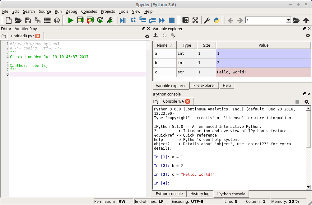
Variable explore

math

We just saw above an example of an import statement. Various tools are available by default in Python or through add-on packages but need to be explicitly brought into your program using import. Here, we’ll use the built-in math module to get access to a variety of standard mathematical functions.

First, let’s import math.

import math

How do we use it? Of course, we can use help, but the output is too long to show here, but dir gives a nice list of what math contains:

dir(math)

['__doc__',
 '__file__',
 '__loader__',
 '__name__',
 '__package__',
 '__spec__',
 'acos',
 'acosh',
 'asin',
 'asinh',
 'atan',
 'atan2',
 'atanh',
 'ceil',
 'copysign',
 'cos',
 'cosh',
 'degrees',
 'e',
 'erf',
 'erfc',
 'exp',
 'expm1',
 'fabs',
 'factorial',
 'floor',
 'fmod',
 'frexp',
 'fsum',
 'gamma',
 'gcd',
 'hypot',
 'inf',
 'isclose',
 'isfinite',
 'isinf',
 'isnan',
 'ldexp',
 'lgamma',
 'log',
 'log10',
 'log1p',
 'log2',
 'modf',
 'nan',
 'pi',
 'pow',
 'radians',
 'sin',
 'sinh',
 'sqrt',
 'tan',
 'tanh',
 'tau',
 'trunc']

A lot of these names ought to look familiar, like sin, exp, and log. All of them live in the math module, and to access them, we can use these functions with the . operator, e.g., math.sin. Here are some examples:

math.exp(2)

7.38905609893065

math.sin(math.pi/2)

1.0

math.factorial(5)

120

A First Program

At this point, we have nearly enough to put together a meaningful program that takes some input information and provides some useful output. Two final ingredients we need are `flowcharts <https://en.wikipedia.org/wiki/Flowchart>`__ and the input function. As our example, we’ll compute the volume of a sphere, which, if you recall, is given by \(V = 4\pi r^3/3\).

Flowcharts

A flowchart is a visual design tool for creating and understanding computer programs. Here, the goal is simply to introduce them as a concept: the program ahead is simple, and so too will be its flowchart. A flowchart for a program to compute the volume of a sphere is shown below.

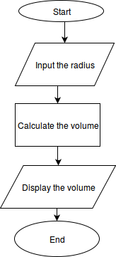
Flowchart for Computing Volume of a Sphere

This simple flowchart highlights a few of the key features we’ll use later on in flowcharts:

• arrows represent the flow of the program from one block to the next
• ovals represent the beginning and ending of a program
• parallelograms represent input from a user or output to a user
• rectangles represent an action taken by the program (which might correspond to several, executed instructions)

We’ll introduce other features of flowcharts as needed throughout the rest of the course. You can create your own flowcharts pretty easily using the online tool draw.io, which was used for the image shown.

Simple Input

All computer programs need some form of input to perform useful tasks. One way to provide a Python program with input directly is by using the input function. The input function can be used to prompt a user to enter information. The information entered is stored as a str and can be assigned to a variable. Here is an example:

my_info = input('Enter your info: ')

Enter your info: 123

Now, my_info is a variable with the value '123'.

my_info

'123'

If we intended to store my_info as an integer value, we would need to modify our code to the following:

my_info_int = int(input('Enter your info: '))

Enter your info: 123

my_info_int

123

The Program

Now, we have what we need and can construct the entire program. Here it is all in one IPython line:

# A short program that computes the volume of a
# sphere given a radius entered by the user.

# Have the user enter the radius and store it as a float
radius = float(input('Please enter a radius: '))

# Import the math module so that we have Pi
import math

# Compute the volume of the sphere
volume = (4/3)*math.pi*radius**3

# Print the volume
print("The volume is ", volume)

Please enter a radius: 2
The volume is  33.510321638291124

One feature of this (and all good programs) is the use of comments, which are lines that start with the # symbol. These lines are not executed by the Python interpreter and, therefore, can be used to describe what various parts of the program do so that a user (or another programmer) can understand the program.

Note: Use comments thoroughly to help you and others understand what your program does.

Finally, we can execute the same program over and over again by saving it as a Python file. Python files are regular text files that, by convention, have the extension .py. Here is a screen capture of this program saved as sphere_volume.py in Spyder. To run the file, one needs to press the green “play” button toward the top, center part of Spyder indicated by the cursor. The results of running the program are shown in the lower right IPython console.

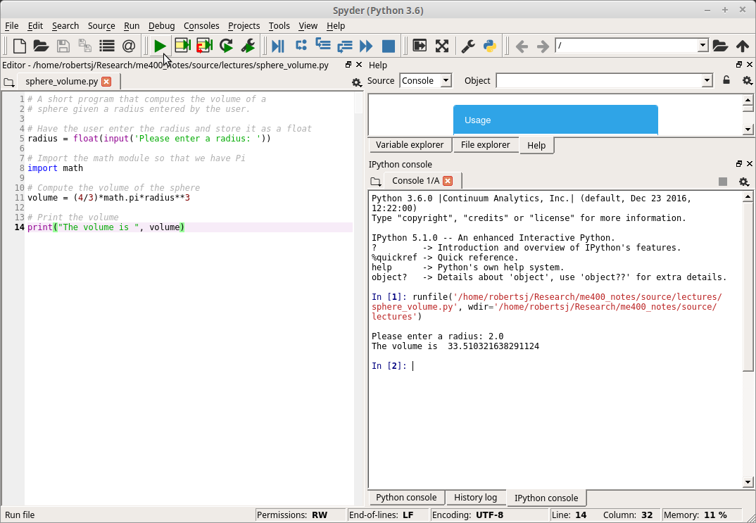
Running Our First Program

Further Reading

This lesson is chalk pretty full of resources linked to throughout and, hence, there are no additional reading required.