Basic Data Processing with NumPy and Matplotlib

Overview, Objectives, and Key Terms

In this lesson, we’ll explore some core features of NumPy and Matplotlib and extend our Python based “calculator” to include processing of arrays of data. NumPy is the basic numerical package for Python. A lot of its utility comes from its numerical, multidimensional array type, ndarray. Use of these arrays in a vectorized way often leads to significantly faster (and much more compact) code. Moreover, the array-valued results of numerical computations are easily visualized using Matplotlib, which was originally developed to provide MATLAB-like graphics in the Python environment.

I think it’s so important that students can create, process, and display data that I highlight it early in the course and revisit it throughtout. NumPy and Matplotlib together provide about the easiest way to work with data.

Objectives

By the end of this lesson, you should be able to

• define and manipulate one-dimensional NumPy arrays
• produce plots of data following best practices
• load data from text files
• save data to text files

Key Terms

• numpy
• ndarray
• np.array
• np.ones
• np.zeros
• np.linspace
• np.sin
• np.mean (or v.mean where v is of type ndarray)
• max (or np.max or v.max)
• sum (or np.sum or v.sum)
• matplotlib.pyplot
• np.loadtxt
• np.savetxt
• v.T, where v is a two-dimensional ndarray
• str formats

from IPython.core.interactiveshell import InteractiveShell
InteractiveShell.ast_node_interactivity = "all"

NumPy and One-Dimensional Arrays

NumPy is not part of Python, but it is a well-supported package. It comes by default in the Anaconda distribution, so you should already have it. Like all packages, we can import NumPy via

import numpy

However, it is far more common to use

import numpy as np

The difference between these approaches is in how we use the numpy module. Built in to numpy are a number of same functions we saw in math, e.g., sin. Hence, we could use numpy.sin(1.0), but if we import numpy as np, we would use np.sin(1.0). I recommend the latter because (1) it is shorter and (2) most online documentation uses the np abbreviation.

Note: Use import numpy as np instead of import numpy.

A Motivating Example

Here’s a common task easily solved using NumPy: evaluate a mathematical function f(x) at discrete points. Why discrete data? Perhaps because that’s all the input data we have, e.g., from measurements, or perhaps we’re trying to plot that function. In any case, this is where NumPy excels. Consider the specific case for which we want to evaluate \(f(x) = \sin(x)\) for \(x \in [0, 1]\), where x is to limited to 10 evenly-spaced points.

Here’s what we need to do. First, always make sure NumPy is imported; in this notebook, we did that above, but here it is again for completeness.

import numpy as np

Now, we create an array x with 10, evenly-spaced points from 0 to 1 using the function np.linspace as follows:

x = np.linspace(0, 1, 10)
x # remember, a variable all by itself as input prints its value as output

array([0.        , 0.11111111, 0.22222222, 0.33333333, 0.44444444,
       0.55555556, 0.66666667, 0.77777778, 0.88888889, 1.        ])

Finally, we evaluate the function np.sin at these points.

y = np.sin(x)
y

array([0.        , 0.11088263, 0.22039774, 0.3271947 , 0.42995636,
       0.52741539, 0.6183698 , 0.70169788, 0.77637192, 0.84147098])

Note that np.sin(x) is used and not math.sin(x). That’s because x in this case is a ndarray, to which the base Python math functions do not apply.

The function np.linspace(a, b, n) gives n evenly-spaced points starting with a and ending with b. Writing the equivalent C++ or Fortran to define such an x is a royal pain; that’s why Python+NumPy (or MATLAB/Octave) is so nice for this type of problem.

Creating and Manipulating 1-D Arrays

We already saw one way to create a one-dimensional array, i.e., np.linspace. There are many other ways to create these arrays. Suppose we have a list of numbers, e.g., 1.5, 2.7, and 3.1, and we’d like to make an array filled with these numbers. That’s easy:

a = np.array([1.5, 2.7, 3.1])
a

array([1.5, 2.7, 3.1])

(It turns out that [1.5, 2.7, 3.1] is actually a Python list, but we’ll cover those later on when we need them; for now, we’ll stick with NumPy arrays exclusively.)

The common ways to make 1-D arrays are listed in the table below.

function	example use	what it creates creates
np.array(seq uence)	np.array([1.5, 2.7, 3.1])	``array([ 1.5, 2.7, 3.1]) ``
np.linspace( start, stop, n um)	np.linspace(0, 1, 3)	``array([ 0. , 0.5, 1. ]) ``
np.ones(shap e)	np.ones(3)	array([ 1.,  1.,  1.])
np.zeros(sha pe)	np.zeros(3)	array([ 0.,  0.,  0.])
np.arange(st art, end, step )	np.arange(1, 7, 2)	array([1, 3, 5])

The table does not tell the whole story of these functions; use help() or the ? mark for further details.

A useful aspect of NumPy arrays is that the basic arithmetic operations of Python (think + and *) apply to such arrays via vectorized operations. For example, two arrays of equal length can easily be multiplied:

a = np.array([1, 2, 3])
b = np.array([2, 3, 4])
c = a*b
c

array([ 2,  6, 12])

Individual arrays can also be operated on by arithmetic operaters. For instance, we could double each element of a by doing

d = 2*a
d

array([2, 4, 6])

Inspecting Arrays and Their Elements

What if we need to get the value of an array element? For example, suppose, as done above, we doubled the array a, called it d, and wanted the first value of d. We need to use array indexing via the operator []. Here’s how we get that first value of d:

d[0]

2

Yes–the first element is accessed using a zero. Python, like C, C++, and many other languages, is based on zero indexing, in which the numbering of sequences starts with zero. Get used to it!

Warning: Numbering starts with zero in Python

By using indexing, we can change the value of d[0], too, e.g.,

d[0] = 99
d

array([99,  4,  6])

The number of elements in an array can be found in two ways. First, we can use the built-in len function:

len(d)

3

We can also use the size attribute, associated with any array, that can be accessed through the . operator:

d.size

3

If we want to access the last element of d, we can use that length directly via

d[len(d)-1]

6

but a much cleaner way to do so is via

d[-1]

6

In fact, by using a negative number, the elements are accessed in reverse starting from the last element. In other words, d[-1] is the same as d[len(d)-1], d[-2] is the same as d[len(d)-2], and so on.

Note: Access the \(i\)th to last element of array via array[-(1+i)].

What else do arrays have to help us? Try using dir!

dir(d)

['T',
 '__abs__',
 '__add__',
 '__and__',
 '__array__',
 '__array_finalize__',
 '__array_interface__',
 '__array_prepare__',
 '__array_priority__',
 '__array_struct__',
 '__array_ufunc__',
 '__array_wrap__',
 '__bool__',
 '__class__',
 '__complex__',
 '__contains__',
 '__copy__',
 '__deepcopy__',
 '__delattr__',
 '__delitem__',
 '__dir__',
 '__divmod__',
 '__doc__',
 '__eq__',
 '__float__',
 '__floordiv__',
 '__format__',
 '__ge__',
 '__getattribute__',
 '__getitem__',
 '__gt__',
 '__hash__',
 '__iadd__',
 '__iand__',
 '__ifloordiv__',
 '__ilshift__',
 '__imatmul__',
 '__imod__',
 '__imul__',
 '__index__',
 '__init__',
 '__init_subclass__',
 '__int__',
 '__invert__',
 '__ior__',
 '__ipow__',
 '__irshift__',
 '__isub__',
 '__iter__',
 '__itruediv__',
 '__ixor__',
 '__le__',
 '__len__',
 '__lshift__',
 '__lt__',
 '__matmul__',
 '__mod__',
 '__mul__',
 '__ne__',
 '__neg__',
 '__new__',
 '__or__',
 '__pos__',
 '__pow__',
 '__radd__',
 '__rand__',
 '__rdivmod__',
 '__reduce__',
 '__reduce_ex__',
 '__repr__',
 '__rfloordiv__',
 '__rlshift__',
 '__rmatmul__',
 '__rmod__',
 '__rmul__',
 '__ror__',
 '__rpow__',
 '__rrshift__',
 '__rshift__',
 '__rsub__',
 '__rtruediv__',
 '__rxor__',
 '__setattr__',
 '__setitem__',
 '__setstate__',
 '__sizeof__',
 '__str__',
 '__sub__',
 '__subclasshook__',
 '__truediv__',
 '__xor__',
 'all',
 'any',
 'argmax',
 'argmin',
 'argpartition',
 'argsort',
 'astype',
 'base',
 'byteswap',
 'choose',
 'clip',
 'compress',
 'conj',
 'conjugate',
 'copy',
 'ctypes',
 'cumprod',
 'cumsum',
 'data',
 'diagonal',
 'dot',
 'dtype',
 'dump',
 'dumps',
 'fill',
 'flags',
 'flat',
 'flatten',
 'getfield',
 'imag',
 'item',
 'itemset',
 'itemsize',
 'max',
 'mean',
 'min',
 'nbytes',
 'ndim',
 'newbyteorder',
 'nonzero',
 'partition',
 'prod',
 'ptp',
 'put',
 'ravel',
 'real',
 'repeat',
 'reshape',
 'resize',
 'round',
 'searchsorted',
 'setfield',
 'setflags',
 'shape',
 'size',
 'sort',
 'squeeze',
 'std',
 'strides',
 'sum',
 'swapaxes',
 'take',
 'tobytes',
 'tofile',
 'tolist',
 'tostring',
 'trace',
 'transpose',
 'var',
 'view']

Several names worth pointing out are dot, max, mean, shape, and sum. The max, mean, and sum functions have pretty intuitive names (and purposes):

d.max()

99

d.mean() # here, (99+4+6)/3

36.333333333333336

d.sum()

109

It turns out that Python has max and sum as built-in functions. Hence, we could instead do

max(d)

99

sum(d)

109

but not mean(d) because mean is not a built-in function. However, mean is a NumPy function, so we could do

np.mean(d)

36.333333333333336

There is no real difference between d.mean() and np.mean(d). My own personal preference is the latter because it looks closer to the programming I first learned eons ago.

The shape attribute is somewhat special; here it is for d:

d.shape

(3,)

Here, the shape indicates a purely one-dimensional array. We’ll see below that shape is a bit more interesting for two-dimensional arrays.

Finally, the dot function implements the dot product, sometimes called the scalar product, for two arrays. In mathematics, we typically refer to one-dimensional arrays of numbers as vectors. For two vectors c and d of length \(n\), the dot product is defined as

\[\mathbf{c} \cdot \mathbf{d} = c_0 d_0 + c_1 d_1 + \ldots c_{n-1} d_{n-1} = \sum_{i=0}^{n-1} c_i d_i \, ,\]

where \(c_i\) is the \(i\)th element of \(\mathbf{c}\). In NumPy, that operation is done via

c.dot(d)

294

or

np.dot(c, d)

294

Of course, knowing how the dot product is defined, we could also use basic element-wise arithmetic coupled with the built-in sum function, e.g.,

sum(c*d)

294

Diving into pyplot

Recall our motivating example: defined x at evenly spaced points, and evaluate np.sin at those points. We printed the points and the function at those points, but it’s often useful to show it via a graph. Matplotlib gives us the tools to do just that. The most common way to import Matplotlib (and, specifically, its pyplot “submodule”) is via

import matplotlib.pyplot as plt

In other words, plt is used as an abbreviation to the longer matplotlib.pyplot.

Note: Just like NumPy is often shorted to np, matplotlib.pyplot is often used as plt.

The most basic plot is very easy to make using plt.plot:

plt.plot(x, y) # x and y were defined above

[<matplotlib.lines.Line2D at 0x7f8865b60dd8>]

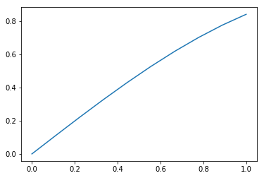
To show the plot, we need to use plt.show:

plt.show()

Multiple Curves and Best Practices

What about multiple curves? Let’s define a second curved equal to np.cos evaluated at x:

z = np.cos(x)

To plot both y and z is also easy, and here, I’ve added a couple extra features that define the basic ingredients needed for a good plot:

plt.plot(x, y, 'k-o', x, z, 'r--x')
plt.legend(['sin(x)', 'cos(x)'], loc=0)
plt.xlabel('x')
plt.show()

[<matplotlib.lines.Line2D at 0x7f8865ae8ba8>,
 <matplotlib.lines.Line2D at 0x7f8865ae8e48>]

<matplotlib.legend.Legend at 0x7f8865af38d0>

Text(0.5,0,'x')

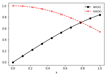
Let’s breakdown the new components. First, consider x, y, 'k-o'. That means y is to be plotted against x, and the line to be used is black (the k), a solid line (the -), and has circle markers (the o). The second curve is defined by x, z, 'r--x'. Here, that plots z against x with a red (the r), dashed (the --) line with x’s as markers (the x). A legend is provided indicating which line is which. The format of the legend always has a sequence of str labels for each line enclosed in []‘s (again, that’s a list in Python, but just follow the syntax for now. By setting loc=0, we’re putting the legend in the best possible place to avoid overlapping with the curves displayed. As a baseline rule, any plot produced should contain an xlabel and either a ylabel (if a single curve) or a legend (if multiple curves).

Note: All plots should include appropriate axis labels and legends.

Some of the available colors, line styles, and markers available in plt.plot are summarized in the tables below.

symbol	color
k	black
b	blue
r	red
g	green
c	cyan
m	magenta

symbol	style
-	solid
--	dash-dash
-.	dash-dot
:	dot-dot

symbol	marker
o	circle
x	x
^	triangle pointed up
>	triangle pointed right
s	square
h	hexagon

In some applications, it can be very important to use a combination of colors, line styles, and markers that produce good looking and easily read graphics when viewed in color and in black and white formats.

Note: Choose good colors, line styles, and markers to ensure excellent contrast in all media.

Data Input and Output via NumPy

For many problems, the data we need to process lives in a file outside our Python code. There are a variety of ways to load data, but NumPy provides an easy way to load data that is in a relatively simple format. Consider a text file that has the following data:

time (s)   vel (m/s)  acc (m/s**2)
0.00000000 1.00000000 0.00000000
0.22222222 1.24884887 0.01097394
0.44444444 1.55962350 0.08779150
0.66666667 1.94773404 0.29629630
0.88888889 2.43242545 0.70233196
1.11111111 3.03773178 1.37174211
1.33333333 3.79366789 2.37037037
1.55555556 4.73771786 3.76406036
1.77777778 5.91669359 5.61865569
2.00000000 7.38905610 8.00000000

The structure is simple: three columns separated by white space. The first row contains information about what the data represent. Here, the columns correspond to times at which the velocity and acceleration of some object are given.

Loading Text Files

Go ahead and save this text in a file. Mine is called data.txt. To load this file, we’ll use np.loadtxt. The basic use of this function is just np.loadtxt(filename), where filename is a str that contains the name of the file. Here, we need just a bit more. In particular, we need tell NumPy to skip the very first row since it contains regular text and not the numbers of interest. Here’s one way to read in that text:

data = np.loadtxt('data.txt', skiprows=1)
data

array([[0.        , 1.        , 0.        ],
       [0.22222222, 1.24884887, 0.01097394],
       [0.44444444, 1.5596235 , 0.0877915 ],
       [0.66666667, 1.94773404, 0.2962963 ],
       [0.88888889, 2.43242545, 0.70233196],
       [1.11111111, 3.03773178, 1.37174211],
       [1.33333333, 3.79366789, 2.37037037],
       [1.55555556, 4.73771786, 3.76406036],
       [1.77777778, 5.91669359, 5.61865569],
       [2.        , 7.3890561 , 8.        ]])

We have the data stored in the variable data. The type looks like an ndarray, but the structure is more like a matrix, i.e., a two-dimensional array—and it is! We can try out the shape attribute again:

data.shape

(10, 3)

That makes sense: we had 10 times at which the velocity and acceleration were provided. 10 rows, and 3 columns. We’ll see next time how to access entire rows and columns of multidimensional arrays, but there is a better way to load in this data directly into three meaningful variables t, v, and a.

t, v, a = np.loadtxt('data.txt', skiprows=1, unpack=True)
t

array([0.        , 0.22222222, 0.44444444, 0.66666667, 0.88888889,
       1.11111111, 1.33333333, 1.55555556, 1.77777778, 2.        ])

Now, we’ve got the times, velocities, and accelerations as three, separate, one-dimensional arrays. With NumPy, loading this sort of data is easy and recommended.

Note: If data is numerical and stored in a simple, collimated format, use np.loadtxt

Like many functions in NumPy and other modules, np.loadtxt accepts quite a large number of optional arguments. You need to use help or the online documentation to learn more (and, of course, you’ll get to explore these in the exercises.)

Saving Text Files

Saving data is just as easy as loading. The function of interest is np.savetxt, and it requires some data and a file name. One way we could save our t, v, and a arrays is via

np.savetxt('output_1.txt', [t, v, a])

Go and check output_1.txt. The data is there, for sure, but it’s not quite the same format that we started with. Instead, t, v, and a were written out in their own row. That’s fine, but often, we want to spit out the data in pretty much the same way we’d like it to be read into our programs.

One issue is that NumPy treats [t, v, a] like an array with a shape of (3, 10), which is exactly how it’s saved to file. Such two-dimensional arrays are basically matrices, and if we want the 3 and 10 reverse, we need the transpose. Here, we can first produce a 2-D array explicitly from [t, v, a] by using the np.array function, i.e.,

data = np.array([t, v, a])
data

array([[0.        , 0.22222222, 0.44444444, 0.66666667, 0.88888889,
        1.11111111, 1.33333333, 1.55555556, 1.77777778, 2.        ],
       [1.        , 1.24884887, 1.5596235 , 1.94773404, 2.43242545,
        3.03773178, 3.79366789, 4.73771786, 5.91669359, 7.3890561 ],
       [0.        , 0.01097394, 0.0877915 , 0.2962963 , 0.70233196,
        1.37174211, 2.37037037, 3.76406036, 5.61865569, 8.        ]])

Then, we need its transpose, i.e.,

data.T

array([[0.        , 1.        , 0.        ],
       [0.22222222, 1.24884887, 0.01097394],
       [0.44444444, 1.5596235 , 0.0877915 ],
       [0.66666667, 1.94773404, 0.2962963 ],
       [0.88888889, 2.43242545, 0.70233196],
       [1.11111111, 3.03773178, 1.37174211],
       [1.33333333, 3.79366789, 2.37037037],
       [1.55555556, 4.73771786, 3.76406036],
       [1.77777778, 5.91669359, 5.61865569],
       [2.        , 7.3890561 , 8.        ]])

That appears to be what we want in our output (if we want it to look like our original input). The only missing ingredient is the first row that indicates what each column contains. Such information can be included by using the header argument. By default, # is appended to the beginning, since np.loadtxt actually ignores lines that start with # (or some other user-specified comment symbol). Here, we can avoid the comment symbol in our output by using setting the comment argument to zero.

Here it all is together:

np.savetxt('output_2.txt', data.T, header='time (s)   vel (m/s)  acc (m/s**2)', comments='')

An Aside: String Formatting

The output is pretty darn close, but the numbers are longer (and they were the first try, too). Behind the scenes, float values are stored with about 15 digits of useful information. When we read in the values from data.txt, they were defined only with 8 digits after the decimal point. You can see that output_2.txt has pretty much the same values, but there are some strange digits out beyond that eight digit. We can limit the output to only 8 digits by using a string format. Consider the following:

print("%.1f" % 0.1234)
print("%.4f" % 0.1234)
print("%.16f" % 0.1234)
print("%.3e" % 0.1234)

0.1
0.1234
0.1234000000000000
1.234e-01

Here, the basic syntact is a str format, which contains a % followed by, e.g., .4f. That means to format the number in normal decimal notation (and not, e.g., scientific) with 4 digits after the decimal point. The last example used an e, which indicates scientific notation (with, here, three digits after the decimal point and before the e). String formatting can be very powerful (and complex). We’ll turn again to the topic again later on, but this gives you a taste!

Saving Text Files: Revisited

Back to our example. Armed with a bit of formatting, here’s the final solution for getting output identical to our original input:

np.savetxt('output_3.txt', data.T, header='time (s)   vel (m/s)  acc (m/s**2)',  comments='', fmt='%.8f')

Inspection of output_3.txt confirms it’s exactly like our original data.txt.

Further Reading

Make sure to explore in depth the help output of all the functions explored in this lesson. Many times, not all function arguments need to be used, but it’s very helpful to know that they exist and what they can help you to do.